INFLUENCE OF RHEOLOGY ON PRESSURE LOSSES IN HYDROTRANSPORT SYSTEM OF IRON ORE TAILINGS

S.yu. Avksentiev ^* and p.n. Makharatkin

Saint-Petersburg Mining University, 199106, St Petersburg, 21st Line, 2, Russia

*Corresponding Author:

S.yu. Avksentiev
Saint-Petersburg Mining University, 199106, St Petersburg, 21st Line, 2, Russia
E-mail: avksentiev@mail.ru

Received Date: 06 April, 2017; Accepted Date: 08 April, 2017

Visit for more related articles at Journal of Industrial Pollution Control

Abstract

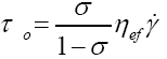
An important trend in mining production intensification, increasing its efficiency and competitiveness in the conditions of modern market relations, is creating a robust transportation basis that could significantly increase the performance of the transportation system with simultaneous reduction of transportation prime cost of minerals and products of their processing. Developing this basis is related to implementing continuous means of transportation among which hydraulic pipeline transport is most common in the mining industry. The calculation of head losses and flow friction characteristic is one of the most important tasks in designing hydrotransport systems. The efficiency of a hydrotransport system depends on solving this task. To reduce the energy consumption and specific amount of metal in a transportation system, mineral processing companies transport processing products in concentrated condition. Such hydraulic fluids are typical of showing initial shear stress ( 0 τ ) and effective dynamic viscosity (ηef), as well as other rheological characteristics that affect the primary parameters of hydrotransport, including head lossess.

Key words

Slurry, Solid particles, Concentration, Head loss, Hydraulic transport, Rheology, Iron ore

Introduction

In ideal viscoplastic fluids (Bingham fluids), viscoplastic properties are conditioned by physical and chemical structure of the fluid when the volume is deformed in the presence of gradient of concentration, temperature and amount of motion, and shear resistance to fluid layers occur. Individual molecular chains change their length and shape. Changing the shape and length of molecular changes causes a plastic layer shear during the initial moment of time, which causes the initial shear stress to occur. When the opportunities of changing the length and shape of individual molecular chains are exhausted, we will see a shear of individual layers of plastic, and the plastic friction law will become effective according to the Bingham model. An example of liquids similar to Bingham plastic are polymers and their solutions (Alexandrov and Kibirev, 2016; Alexandrov, et al., 2012).

Methods

When mixing a liquid continuous and solid discrete medium, a new continuous medium is formed, a suspension with the properties differing from its components taken separately. Every particle of the small-fraction solid phase in the aqueous medium receives a liquid shell on its surface, which results in a dipole to be formed that carries a positive and negative charges. The dipole orientation in the fluid volume is defined by their interaction. As a result of this interaction, a structure is formed and the suspension can be regarded as a continuous media. When the force F acts on the volume of this fluid, solvate shells of dipoles are initially deformed and the initial shear resistance occurs, which in this case is caused by an elastic strain. Individual layers of the hydraulic fluid are sheared and the plastic viscosity occurs. This mechanism of viscoplastic properties demonstration is typical of the fluids that include small and almost homogeneous particles, such as kaolin hydraulic fluid.

Real fluids include particles of small classes, but heterogeneous in shape. Therefore, some solid particles will not be fully covered with a solvate shell or will lose it. In case of volume deformation of this suspension, viscoplastic friction is added by purely mechanical friction of particles that have lost it or failed to obtain solvate shells on its surface. The viscosity in these fluids is manifested as a total effect of plastic viscosity caused by the shear resistance of individual hydraulic fluid layers and by the friction resistance of solid particles that have no solvate shells. Consequently, viscoplastic properties in the volume of suspensions are related to their physical (dipole formation) and mechanical (friction) nature. In accordance with this model of viscoplastic friction occurrence, occurring resistances can be associated with some effective (apparent) viscosity according to the formula (Darcy, 1957).

(1)

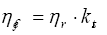
Where effective viscosity (viscosity from total effect), coefficient structure.

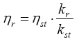
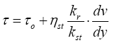
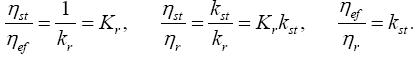
Consequently, the viscosity coefficient depends on the structural viscosity that will be associated with the effective viscosity through the following ratio:

(2)

Where -plastic viscosity coefficient.

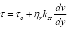
Every component of effective viscosity is defined by its own shear angle (Figure 1).

Due to the abnormal (in relation to the Bingham model) manifestation of plastic properties, such fluids can be referred to a class of Bingham pseudoplastics (Heywood and Richardson, 1978).

As the concentration of solids grow, the Newton viscosity increases, and at some limit concentration, structural properties occur in the hydraulic fluid volume, viscosity appears, along with the initial shear resistance (Heywood and Alderman, 2003).

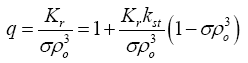
The ratio between plastic and structural viscosity is determined from the formulas (1) and (2), where we obtain

(3)

The effective viscosity expresses a mean viscosity and is a function of the mean concentration of solid particles and the suspension flow cross-section. The structural viscosity is manifested in case of plastic deformation of the hydraulic fluid volume at the border of the flow core, and it is constant in magnitude and has the maximum value (Kumar, et al., 2015). The plastic viscosity effect occurs in case of the deformation of hydraulic fluid layers and depends on the structural viscosity in its value. 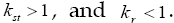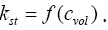The formulas result in If , then and, consequently , e.g., in this case, the hydraulic fluid represents a pure liquid. The structure coefficient value, as well as the values of effective viscosity components, is defined by the concentration of solids of the tail pulp, e.g.,

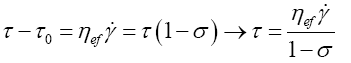
With respect to specific features of how viscoplastic properties of highly concentrated small-fraction hydraulic liquids considered above manifest themselves, the Bingham model for them can be as follows:

(4)

or through the structural viscosity

(5)

The models (4) and (5) differs from the Bingham- Shvedov model in that the effective viscosity considers both structural and plastic properties of the deformed volume of the fluid medium (hydraulic fluid).

Hydraulic fluids of tailings are formed when fine particles of iron ore are mixed with the liquids phase-water. The primary properties of formed hydraulic fluids depend on the number of particles in the volume of water accommodating them. In case of small concentrations of solids, the hydraulic fluid slightly differs from the standard Newton liquid, and the model of this suspension is the Newton viscous friction law (Schmitt, 2004).

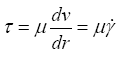(6)

Where suspension dynamic viscosity coefficient, velocity gradient upon the pipeline crosssection, dv =infinitely small change of the suspension flow velocity towards an infinitely small change of the flow radius dr .

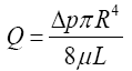
Integrating the equation (6) results in the known Hagen-Poiseuille formula for the liquid flow

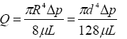(7)

or for the mean flow velocity

(8)

Where R =internal pipe radius, Δp =pressure difference in the selected pipe section L long, d = 2R =internal pipe diameter.

The dynamic viscosity coefficient is expressed from (9).

(9)

The last equation can be represented as follows:

In the numerator of the equation (10) there is the expression for the tangent shear stress on the pipeline wall, and in the denominator, is the expression for the shear rate gradient

(10)

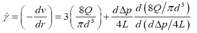
Taking into account that the volumetric flow rate in the pipe cross-section is proportional to the man linear flow velocity and the pipe cross-section area, we obtain as follows for the shear rate gradient

(11)

The reduced expressions are true for vicious fluids whose flows in laminar conditions result in resistances conditioned by tangent stresses in accordance with the Newton friction law (Portable Surface Roughness Tester Surftest SJ-210 Series, 2014).

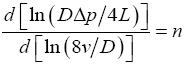
As the concentration of solids increases to some limit value, a spatial structure is formed in the suspension volume, with somewhat organized orientation of particles upon the pipeline cross-section. The hydraulic fluids rheological characteristics start differing from their values in case of a simple vicious friction. For this case, we can use the solution (Nikuradse, 1932) relative to the shear rate gradient:

(12)

that will look as follows when substituting

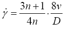(13)

Where D =internal pipeline diameter.

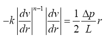
With respect to these transformations, the initial equation of the shear stress dependency from the deformation rate will look as follows:

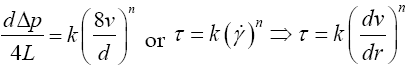(14)

The last expression defines the connection between shear stresses on the pipeline wall in the laminar flow area for liquids and hydraulic fluids differing in rheological parameters from Newton liquids. k coefficient is viscosity (pseudoviscosity) with the size of which makes this parameter different from the Newton fluid viscosity coefficient. The exponent of power n in the equation (13) defines the flow curve inclination angle to the axis in logarithmic coordinates and, respectively, shows the difference of this non-Newton liquid from the Newton one and is referred to as the structural number.

The formula (14) is referred to as the Ostwaldde- Valle rheological model and describes the dependency of tangent shear resistances from the deformation rate gradient for an exponential friction law. The structural number is and can be defined by means of viscometric experiments.

To define the connection of parameters k and n , we should transform the shear stress equation into which allows changing the formula (14) as follows

(15)

Since it means that 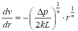(16)

By integrating this equation with the limit condition of meaning that the liquid velocity on pipe walls equals zero, we find the velocity distribution law

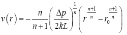
The maximum flow velocity is achieved on the pipe axis (r = 0):

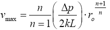(17)

The liquid flow rate will be calculated under the formula

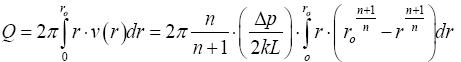(18)

After integration, we obtain as follows

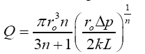(19)

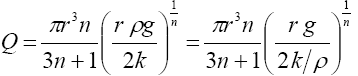
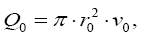
For a full pipeline cross-section when r₀ = R, the flow rate in the pipeline will be

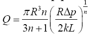(20)

that is transformed into the Hagen-Poiseuille in case of n = 1

If we introduce the cross-section mean flow velocity and a generalized number of Re*, in accordance with the equalities 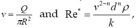the liquid flow rate formula under the Ostwald-de-Valle model can be recorded as the Darcy-Weisbakh law, e.g., through the hydraulic resistance coefficient

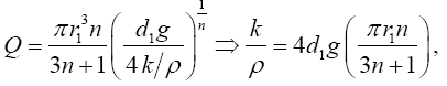
To apply the Ostwald-de-Valle model in practice when calculating the flow of hydraulic fluids, we can use experimental viscometric data obtained with a capillary viscosity gage. The principle of action of these viscosity gages is based on determining the time of free flow of the fixed portion of the tested hydraulic fluid from the gage's chamber through a narrow cylindrical pipe (capillary) (Furlan and Visintainer, 2014).

By replacing the pressure gradient in the formula (20) with a value of , we obtain as follows:

(21)

From the formula (21), we see that when the specified volume of the investigated liquids completely flows through Ostwald viscosity gage capillaries with the radii of r₁ and r₂ , the following relation will be true

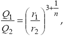
Since the relation between outflow rates is reversely proportional to the period of outflow, we obtain as follows

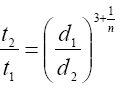(22)

Where t₁ and t₂ =period of outflow through capillaries with r₁ and r₂.

The structural number of n is calculated under the formula (22). The second constant (apparent viscosity) of k is defined from the formula (23).

(23)

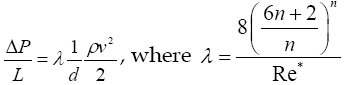
Now we can calculate the coefficient of hydraulic resistances λ and pressure loss

In this manner, when the concentration of particles in the hydraulic fluid volume increases, the liquid model transforms into the exponential liquid model corresponding to the Ostwald-de-Valle model that is generalized as related to the Newton mode, since the latter is transformed into the Newton model when the structural number The concentration of solids when viscoplastic properties occur that correspond to the Ostwald-de-Valle exponential model is a limit (or critical) concentration- ccr 1. The limit concentration value c_{cr 1} can be defined based on experimental data. The initial shear starts manifesting, and the viscous liquid model is transformed into the Shvedov-Bingham model (Figure 2). The parameter values included into the rheological equation (23) depend on the concentration of solids in the fluid flow. For some concentration values, the initial shear stress becomes zero, as well as the structure coefficient. In this case, the equation (23) is transformed into the equation for Newton liquid. The equation shows that when the viscoplastic fluid flows through a pipelinein diameter, the fluid flow is divided into two zones:

- flow core characterized by the initial shear resistance of the flow core radius of and some crosssection mean concentration of solids

- annular flow between the flow core and the pipeline wall, e.g., flow in the gap limited by internal radius and external radius so that the thickness of the annular flow zone equals The concentration of particles in the annular flow changes from the maximum mean value of at the boundary of the flow core to zero on the pipeline wall (Yagi, et al., 1972).

The fluid flow schematics in the pipeline crosssection are given in Figure 3.

The relative dimensions of flow areas (flow core and annulus) depend on the concentration of solids. When the concentration decreases, the flow core is also decreased or may even disappear at some point. The entire pipeline cross-section is occupied by the annular zone, and the effective viscosity becomes equal to the plastic viscosity.

The structure coefficients change from 1 (at minimal concentration) to some maximum value when the concentration is decreased. For the limit values of concentration, the structure coefficient formula may be represented as follows:

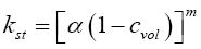(24)

Where is a coefficient whose numerical value depends on the limit concentration value c_{cr 1}

when the core is formed, m is a coefficient describing mechanical properties of a solid material.

In accordance with the formula (24), the structure coefficient k_st equals as follows:

For the concentrations equal to the limit value, the flow structure starts to form, and the primary impact on the flow will be originated from the plastic properties of the fluid and the viscosity in accordance with the Ostwald-de-Valle model.

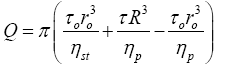
Figure 3 shows that the total flow rate of the hydraulic fluid through the pipeline cross-section will be equal to the sum of flow rates in the flow core and in the annular zone, e.g.,

(25)

Where Q=total flow rate in the pipeline; flow rate in the central area (in the flow core);Q _r -flow rate in the central area of the flow.

By expressing the flow rate through the flow velocity and the cross-section, we obtain as follows:

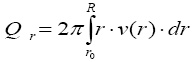(26)

Where fluid velocity in the flow core, flow velocity in the annular area that is a function of radius.

To determine the change law for velocities and v(r) , we will consider forces acting on the fluid flow elements (Figure 4):

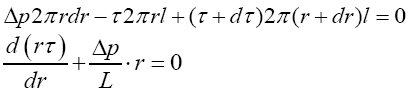(27)

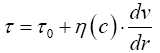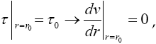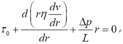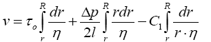
Let us record the Shvedov-Bingham equation and differentiate it for the limit values of tangent stresses then from which we will obtain after dividing variables: 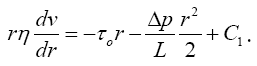By solving the equation in relation to the velocity , we will obtain the following equation

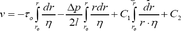(28)

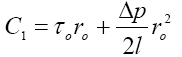
The integration variables C₁ and C₂ are defined with respect to the limit conditions: and will be as follows for constant C₂:

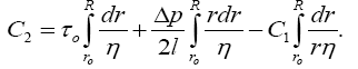
By substituting the obtained value of C₂ in the velocity formula, we will determine C₁ constant:

The final law of flow velocity change in the pipeline cross-section will be as follows

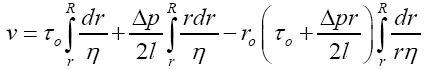(29)

The final integration of the equation (29) will result in the following hydraulic fluid flow rate formula

(30)

Let us reduce the formula to a non-dimensional form by dividing it by parameter 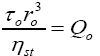and by taking the ratio of we will obtain:

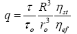(31)

Let us denote and record as follows, in accordance with (30), (31):

As a result, the formula (31) will be the following non-dimensional function:

(32)

Where is denoted.

The formula shows that the average flow rate of the hydraulic fluid is defined by the flow core radius, the shear stress and the viscosity in flow areas. Each of these zones is characterized by its viscosity value. The equation (32) is a final view of the mathematic model of the process expressed in a non-dimensional form. It follows from the equation that for 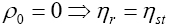and, consequently, the continuum represents a pure liquid; for 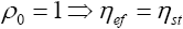and the continuum is expressed by a solid body.

Taking into account that the relative stress is a relation between the initial shear resistance and the total shear resistance on the pipeline wall, and referring to the rheological model of the suspension flow, we can record it as follows:

(33)

or, for the initial shear resistance,

(34)

The formulas (33) and (34) are easily transformed into the expression for pressure losses along the pipeline length if we record the shear stress through normal stress originated from the pressure difference:

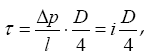
Where i = pressure losses along the pipeline length, Pa/m.

By substituting the expression for the shear resistance in the formula (34), we will obtain a formula for pressure losses:

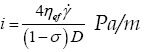(35)

On the other hand, and where i_f = head losses along the pipeline length, m; fluid density, kg/m³.

It means that the head losses can be recorded as the formula

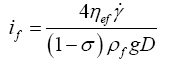(36)

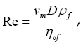
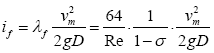
By replacing the velocity gradient of with a respective expression, and the dynamic coefficient of effective viscosity with the expression through the Reynolds value, e.g.:

Which will result in the following dependency after substituting in the expression (36)

In the general form, the head losses can be calculated under the Darsy formula

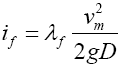
By comparing the expressions, we get a formula for hydraulic resistances in the flow of a viscoplastic hydraulic fluid

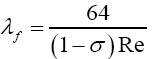(37)

Where 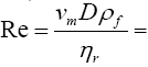critical Reynolds value for laminar flow conditions.

Results

The resulted formula for hydraulic resistances differs from the known dependence for the laminar flow of pure liquids in that its numerator has a parameter characterizing the stressed condition of the hydraulic fluid expressed by the relation of the initial stress to the total shear stress (Vasylieva, 2015; Ryabinin and Trukhanov, 2015).

The formula shows that as the relative stress increases, so does the coefficient of hydraulic resistances.

The formula (37) also shows that theoretical investigations and resulted dependencies do not contradict with known and commonly accepted models of suspension flow and at the same time, it takes into account the dependency of hydraulic resistances on the viscoplastic properties of the hydraulic fluid defined by relative shear stress

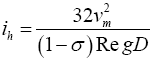
In the final form, the head losses in the flow of concentrated hydraulic fluids having viscoplastic properties are defined under the following expression

(38)

Where average flow velocity of the hydraulic fluid.

Discussion

When designing hydrotransport systems, the issues of solids concentration in a hydraulic fluid flow must be solved, which will result in the lowest possible energy consumption. The expenses for hydraulic transportation of solid materials are a complicated function of mechanical characteristics of solid phase and hydraulic fluid. The resulted method to determine head losses and the hydraulic resistance coefficient based on the rheology of iron ore suspension of tailings can be used in developing a system for hydraulic transportation of iron ore tailings.

The determinants in the formula (38) are the fluid viscosity and the concentration of solids that are defined experimentally.

Conclusion

The obtained methodology to determine head losses and the hydraulic resistance coefficient based on the rheology of iron ore suspension of tailings can be used in designing a hydraulic transport for iron ore tailings.

1. The calculation has shown that the results of analytical dependencies of determining head losses and the hydraulic resistance coefficient can be taken for analysis and determining the losses along the length of non-newton liquids.

2. When the solid phase concentration in iron ore tailings hydraulic fluid increases, we can consider both viscoplastic liquids with initial shear stress ( τ₀ ) and effective dynamic viscosity (η ) according to the adopted Bingham-Shvedov model.

3. When the solid phase concentration in a hydraulic fluid flow increases during transportation of a specific volume of solids, the specific amount of metal in the pipeline system is reduced to the decreased required pipeline diameter.

References

1. Alexandrov, V.I. and Kibirev, V.I. 2016. Assessing the efficiency of applying polyurethane coatings of hydrotransport pipelines as compared to steel pipelines. Enrichment of ores. 6 : 41-45.
2. Alexandrov, V.I., Avksentyev, S.Y. and Gorelkin, I.M. 2012. Specific energy efficiency of hydraulic transportation of minerals processing products. Enrichment of ores 3 : 39-42.
3. Darcy, H. 1957. Experimental research on the motion of water in pipes. Paris: Malet-Bachelier.
4. Furlan, J.M. and Visintainer, R.J. 2014. Centrifugal pump performance when handling highly non-Newtonian clays and tailings slurries. In 19th International Conference on Hydrotransport 2014, Golden, 24-26 September 2014. 117-130.
5. Heywood, N. and Richardson, J. 1978. Head loss reduction by gas injection for highly shear-thinning suspensions in horizontal pipe flow. In Proceedings of Hydrotransport 5 Conference, BHRA Fluid Engineering, Cranfield, U.K. 1 : 146-152.
6. Heywood, N. and Alderman, J. 2003. Developments in slurry pipeline technologies. Chem. Eng. Prog. 4 : 100-107.
7. Kumar, U., Singh, S.N. and Seshadri, V. 2015. Bi-modal slurry pressure drop characteristics at high concentration in straight horizontal pipes. Int. J. Eng. Tech. Res. 3 : 394-397.
8. Nikuradse, J. 1932. Law of turbulent flow in smooth pipes. Düsseldorf: VDI-Verlag.