
ISSN (0970-2083)
ISSN (0970-2083)
Samad Jafarmadar1 and Alireza Shayesteh Nezhad2*
1Department of Mechanical Engineering, University of Urmia, Urmia, Iran
2Oil & Gas Department, National Iranian South Oil Company, Ahwaz, Iran
Received date: 07 March, 2015 Accepted date: 04 June, 2015
Visit for more related articles at Journal of Industrial Pollution Control
The purpose of this research is to study the emission and dispersion of hydrogen sulfide gas (H2 S) from elevated flare in Aghajary compression station. This flare is used only during shut-down or start-up. This flare has ignition system, when the feed gas discharged to the flare will be ignited by sparks. It is very likely that the ignition system does not work or ignition is delayed. In this situation H2 S may come down to the ground level and if it's concentration be greater than 8 ppm it can endanger human health and lead to death. Gaussian-based dispersion models are widely used to estimate local pollution levels. The accuracy of such models depends on stability classification schemes as well as plume rise equations. A general plume dispersion model for a point source emission, based on Gaussian plume dispersion equation, was developed. A mathematical model formulated in a computer program written in Pascal language was utilized in finding the ground level concentrations of H2 S emitted from the elevated flare and final results compare with PHAST software results.
Elevated Flare, Dispersion , Hydrogen Sulfide, PHAST, Gaussian Model
Air pollution is dangerous problem facing humans, and it caused great harmful which may cause death especially when it is higher than the critical environmental limits of pollutants. Oil and gas activities is one of the most important pollution source and very toxic gas emitted in environment in this industry. A large number of oil reservoirs have hydrogen sulfide gas in their components. H2S during the oil processing is separated from oil, if there are processing facilities sent to refinery otherwise discharge to flare for burning, as well as in shut down and stat up usually gas sent to flare. The flares system is safety equipment necessary in petroleum plants. Flares are designed to avoid the uncontrolled emissions. It is used for two cases related strongly with safety, one of them is during the unstable operations such as start-up, shutdown of unit operations; the second case is to management the waste gases discharged from routine production operations. Elevated flare is a one type of flares, it is a vertical pipe opened from its top supplied with igniters.
The waste or discharged gases are burned with atmospheric air at the tip of flare stack.Aghajary compression station is located in south of Iran, it's flare is elevated type with ignition system and during uncontrolled process or in shut down and start-up is used.In this investigation dispersion of H2S emitted from this flare at ignition failure has been study. Gaussian model written in Pascal language and PHAST software is used for gas dispersion study . The programmed model and software model takes into consideration the meteorological conditions (wind speed, ambient temperature, and atmospheric stability) which may take place at the study region. According to OSHA standard the maximum H2S allowable ground level concentration(MGLC) for 8 hours working is 8 ppm and for 10minutes is 20-50 ppm and 100 ppm dangerous for life Health immediately. Table1 shows the feed gas composition and specifications of flare and ambient condition are shown in Table 2.
One of the research at this case belong to Hatam Asal Gzar and Khamaal Muhsin Kseer (2009) in this research they studied pollution emission and dispersion from several flare in Iraq by using Gaussian model. Seema Awasthi, Mukesh Khare and Prashant Gargav (2006) studied the pollution dispersion of power plant flare by using Gaussian model.
Theoretical Basis of dispersion air pollutants emitted from flares
Mathematical model formulating in a computer program written in Pascal language using Gaussian equation is utilized to investigate the dispersion process and distribution of pollutants (H2S) emitted from the elevated flare. With Gaussian equation(1) the ground level concentrations of H2S is determined.
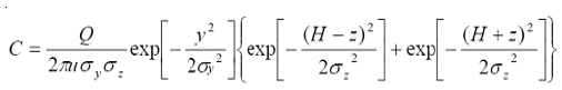 (1)
(1)
Where,
C : Air pollutant concentration in mass per volume (g/m3)
Q : Pollutant emission rate in mass per time (g/s)
u : Wind speed at point of release (m/s)
y : Crosswind direction standard deviation of the concentration distribution at downwind distance x
z : Vertical direction standard deviation of the concentration distribution at downwind distance x
y : Horizontal distance from plume centerline (m)
H : Effective height of the centerline of the pollutant plume
z : Vertical distance from the ground level (m)
The Maximum Ground Level Concentration (MGLC) is usually of interest. It will occur at some downwind distance right below the centerline of the plume ( y = 0, z = 0) then Eq. ( 1) is reduced to:
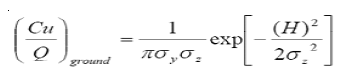 (2)
(2)
Correlation for MGLC
Using Eq. (2) to calculate MGLC requires one to generate repetitious solution. In order to approximate MGLC, without calculating Eq. (2), many times a correlation formula has been generated by using the MGLC graph presented in the Workbook is been used]. The values of the constants are listed in Table 3.
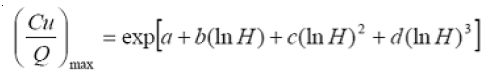 (3)
(3)
Where,
(Cu/Q)max : maximum ground level concentration a,b,c,d : Coefficients for a given stability condition
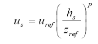 (20)
(20)
Where p is the wind profile exponent. Values of p may be provided by the user as a function of stability category and wind speed class.
Comparison between computer program model and PHAST model is with neutral stability condition is presented in figure 5 and 6. There is good match between the two models and maximum deviation is about 11%. As is clear from these graphs after short distance from flare concentration become 1/3 and after that With a lower slope decreases As well as with increasing wind velocity mixing length decreases too.
Fig. 4 H2S centerline concentration with u=4 m/s
Fig. 5 H2S centerline concentration with u=8 m/s
As previously mentioned, it is very important we find MGLC for this purpose 32 different cases defined. Each case has special meteorological conditions with 45 and 70(m) flare height. We look for with which condition MGLC is greater than 8 ppm until necessary instruction to be considered. For reach our goal three stability condition, very unstable, neutral and very stable with various wind velocity are considered. All of these condition occur during the year. Tables 5 and 6 are shown MGLC and it’s distance(xmax) for two flares.
As results at neutral condition for two flare MGLC is zero and in this condition operators have enough time to stop the operation and for other weather condition, A(very unstable) and G(very stable) MGLC not zero but concentration flare with 70 m height not greater than 8 ppm thus operator do not do any thing but it is better to end the operation for the first time. The height of Aghajary flare is 70 m and another flare with 45 m height consider for second alternative, if it is possible the height of flare reduced however, for second flare MGLC equal 8 and in situation 8 hours existing for reaction.
Other important result is, increasing wind velocity in very unstable(A) condition decrease the xmax and MGLC but in very stable(G) condition wind velocity increasing, decrease MGLC and increase xmax.
Contour of H2S distributing at several cases are shown in following Figures.
Other results that can be achieved graphs about mixing length and downwind distance, at A,D and G weather conditions with increasing wind velocity mixing length is reduced but for cloud length at A condition reduction is seen and at D and G increasing. Generally, maximum cloud height in the neutral weather condition and minimum in the very stable condition, cloud height in the very stable condition is very greater than other conditions at a equal wind velocity an minimum was occurred at very unstable condition.
Because of the gas reached to the ground level at stability condition A and G, study other rang of wind velocity were important Therefore the problem was resolved for wind velocity less than 4 m/s and the results are shown in Table 7.
As is clear from the results at stability condition A with decreasing wind velocity MGLC decreased and xmax increased but the important results obtained at th G stability. In very stable condition with decreasing wind velocity MGLC increase quickly and very close to the flare (xmax=49 m) MGLC be 100 ppm and this mean is death for each alive creature.
For further information some contour from critical cases are given below.
Authors thank National Iranian oil company (NIOC) and National Iranian South oil company(Nisoc) for their help and financial support.
Copyright © 2026 Research and Reviews, All Rights Reserved