COMPARATIVE STUDY BETWEEN GENETIC ALGORITHM AND NEURAL NETWORK COUPLING AND MONITORING TOOLS ON THE DISPERSION OF POLLUTANTS FROM THE YASSA-DIBAMBA THERMAL POWER PLANT

A. C. Goune¹, J. C. Seutche^2*, R. Y. Ekani³, B. E. Essombo⁴, J. L. Nsouandele⁵, G. H. Ben-Bolie⁶

^1,2,4Research and Training Unit of Physics, Energy, University of Yaoundé I- Cameroon, Yaoundé, Cameroon

³Department of Energetics Engineering, Energy, University of Douala, Research and Training Unit of Physics, Cameroon

⁵National Advanced Scholl of Engineering Maroua, University of Maroua Cameroon, Maroua, Cameroon

⁶Department of Physics, University of Yaounde I, Laboratory of Atomic, Moleculary and Nulear Physics, Yaounde, Cameroon

*Corresponding Author:

J. C. Seutche
Research and Training Unit of Physics, Energy, University of Yaoundé I- Cameroon, Yaoundé, Cameroon
E-mail: sejial8002@gmail.com

Received: 10-Mar-2023, Manuscript No. ICP-23-91340; Editor assigned: 14-Mar-2023, PreQC No. ICP-23- 91340 (PQ); Reviewed: 28- Mar-2023, QC No. ICP-23-91340; Revised: 03-Apr-2023, Manuscript No. ICP-23- 91340 (R); Published: 10-Apr-2023, DOI: 10.4172/0970-2083.002

Citation: Goune AC, Seutche JC, Ekani RY, Essombo BE, Nsouandele JL, Ben-Bolie GH. Comparative Study between Genetic Algorithm and Neural Network Coupling and Monitoring Tools on the Dispersion of Pollutants from the Yassa-Dibamba Thermal Power Plant. J Ind Pollut Control. 2023;39:002.

Copyright: © 2023 Goune AC, et al. This is an open-access article distributed under the terms of the Creative Commons Attribution License, which permits unrestricted use, distribution, and reproduction in any medium, provided the original author and source are credited.

Visit for more related articles at Journal of Industrial Pollution Control

Abstract

Prediction plays an important role in air quality monitoring. However, nowadays, the main difficulty is to accurately predict the impact of pollution sources on the environment due to atmospheric dispersion models that are not accurate enough. To solve these problems, this paper proposes a coupling between an optimisation model and a prediction model. In this work, a Genetic Algorithm Coupled With Neural Networks (GA-ANN) was used to predict the concentration of pollutants in the Yassa region. Thus, the genetic algorithm was used as an objective function optimisation tool and the neural networks were used as a data learning tool to predict the concentration values. The model takes into account the meteorological parameters of the study area and the source over 5 years, from January 2017 to December 2021. To evaluate the model, two indices are used to indicate the performance of the prediction model; the squared correlation coefficient R2 whose value in the test case is about 0.88 and the Root Mean Square Error (RMSE) whose best value is about 0.0044. We also evaluated the optimisation methods and found that compared to the particle optimisation swarm, the genetic algorithm gives a better “Fitness Function Curve” as a function of the number of iterations. The results show that the GA-ANN coupling is more accurate and efficient in estimating pollutant concentration values than CFD and the Gaussian model

Keywords

Neural network, Genetic algorithm, Concentration, Pollutant dispersions, Prediction, Optimization

Introduction

Nowadays exposure to air pollution is the leading environmental risk factor in relation to adverse health impact (Liu, et al., 2017; Apte, et al., 2015). Particulate Matter (PM₁₀, PM_2.5 i.e. diameter less than 10 and 2.5 ), Nitrogen Oxide (NOX) are components that dominate ambient air pollution associated with urban development leading to an increase in temperature due to industrial activities, especially thermal power plants (Lin, et al., 2018;Li, et al., 2017; Andre, et al., 1999). In Cameroon, regulatory measures have been taken to reduce the quantity of pollutants in the atmosphere, in particular the ones regulating the quality of the air in Cameroon(Li, et al., 2018; Konga, 2005; EPESS). This is backed by law n°96/12 of August 1996 relating to the management of the environment of the decree n°2011/2582/PM fixing the modalities of protection of the atmosphere. However, given the complaints of the population, the challenge remains high in areas with thermal power plants close to sensitive receptors, such as the thermal power plant of Yassa-Dibamba (heavy fuel oil) which emit pollutants such as Carbon Monoxide (CO), Nitrogen Dioxide (NO₂), Sulphur Dioxide (SO₂) and Particulate Matter (PM₁₀) known for their adverse impacts on human health (Roemer, et al., 2000; Middleton, et al. 2008). Achieving a target depends on the behavior of pollutants from these sources (Lemiere, et al., 2001). To meet air quality standards in sensitive receptor areas, an assessment of the impact of pollutant emissions must be performed. Two ways are possible: By direct measurement through site monitoring or by using an “Atmospheric Dispersion Prediction Model” (Pascal, et al., 2011). Considering the fact that monitoring sites are not accessible in our country due to our low purchasing power, the predictive study of pollutants in sensitive receptor areas is necessarily done with dispersion modelling, which is an effective tool for behaviour of pollutants in space and time at the local scale (Ministry of Sustainable Development, the Environment, 2017). The prediction of air quality is very essential not only to control the variation of air quality but also to provide timely information on the quality of the environment (Pournazeri, et al., 2014; Yang, et al., 2015; Corani, et al., 2016 ; Wakeel, et al., 2017; Van fan, et al.,2018; Yang, et al., 2018).

Several researchers have worked on the modelling of air pollutant dispersion, with successful atmospheric dispersion simulation models including the: Gaussian, Lagrangian and Computational Fluid Dynamics Models (CFD). The Gaussian model has a simple mathematical expression, needs only a few parameters and is used in operational cases because the results are obtained quickly. This is however not accurate enough (Hanna, et al., 1982). Compared to the CFD and Lagrangian model, the Gaussian model is fast in computation time but less efficient in prediction results. Therefore it is necessary to have a fast and accurate model to improve the quality of the results (Bieringer, et al., 2015). In the literature, several works have been presented on the modelling of atmospheric dispersion, one of the objectives being to have accurate and operational results for an effective and rapid prediction of atmospheric dispersion of pollutant. This is the case of (Florian, 2011). In his work he uses the “Flow’air-3D” approach based on the constitution of CFD wind data calculated on the industrial site and a SLAM modelling code. The couple Flow’air-3D/ SLAM, by combining accuracy and speed has allowed to represent in a satisfactory way the dispersion on a complex case, however the model is adapted to a single site. Pierre used in their work Cellular Automata (CA) as rule of transition from one cell to Another And Neural Networks (ANN) for the modelling of the atmospheric dispersion of the methane puff (Pierre, et al., 2016). The objective of combined CA-ANN is to predict accurately and quickly the evolution of a puff of substance, however this model has limitations because we observe an increase in error with the number of iteration, the neural network used recurrent type seems to become unstable during modelling. In order to effectively monitor the emissions of hazardous gases from pollution sources, developed a method for dispersion prediction and source estimation quickly and accurately based on neural networks, particle swarm optimization and expectation maximization (Sihang, et al., 2018). Where neural networks are used for the accurate and efficient prediction of concentration distribution, particle swarm optimization and expectation maximization are applied to estimate source parameters that effectively accelerate the convergence process. Bin proposed a new model for the estimation of a hazardous source by developing the artificial neural networks coupled with the hybridization of particle swarm optimization and simulated annealing algorithm (Bin, et al., 2018). Where the neural networks were used to predict the dispersion and the simulated annealing method was used to improve it to global search. The results illustrate that the proposed method is capable of estimating the hazardous sources and the wind field accurately. Rongxiao had solve the serious public health problem caused by pollutants from production industries (Rongxiao, et al., 2018). They also worked on the prediction of contaminant dispersion in order to control the emissions and used a model integrating neural networks and AERMOD system, with the neural network that predicted the dispersion and the AERMOD system that was used to bring data for prediction needs, the results showed that the model was indeed feasible for contaminant prediction. However, the model still underestimates the concentrations. Juan proposed a Semi-Empirical Model (SEM) to improve the accuracy of vapor intrusion estimates by specifying pollution scenarios (Juan, et al., 2022). For this article we replaced the previous models by the Genetic Algorithm and Neural Network Coupling (GA-ANN), which has shown some qualities. The main objective of this work is to evaluate the coupled genetic algorithm-neural network model by comparing it to the operational field tool and other prediction model

Location of Study Area

The Yassa-Dibamba Thermal Power Plant is located on the Douala-Yaoundé heavy axis, more precisely at the entrance of the city of Douala and a few meters from the bridge over the Yassa-Dibamba between 3° 59’ 44’ N and 9° 49’ 10’ E, in the subdivision of Douala 3rd which has a population of about 1,020,061 inhabitants (Seutche, et al., 2019; Seutche, et al., 2012). The Yassa- Dibamba thermal power plant is built in 2008 on approximately 4 hectares (ha) in an overall area of approximately 7.7 ha. It has an installed capacity of 88 MW, with an available capacity of 86 MW. The thermal power plant is equipped with eight generators, and each generator is equipped with a WARTSILA 18V38 diesel engine (Fig. 1).

Figure 1: Location map of the Yassa-Dibamba thermal power plant.

The 5-year meteorological data for the central region comes from the Douala airport station, available at the National Meteorological Department. We present the temperature from January to December of the year 2017 to 2021 (Fig. 2). It can be seen on the figure that July, August, September 2020 and July, August 2021 are the months with the lowest temperature with T=26°C and February 2019 is the month with the highest temperature with T=32°C.

Figure 2: Temperature of the month of the year. Note: () 2017; ()2018; () 2019; ()2020; ()2021.

The wind rose is important for predicting the direction of pollutants in the atmosphere (Fig.3). The meteorological data has been collected from the meteoblue website. During the study period, the dominant wind direction southwest.

Figure 3: Wind rose diagram for study period of Yassa.

The curve shows the evolution of the wind speed between January 2017 and December 2021 (Fig. 4). It is observed that March 2019 is the month with the highest wind speed with V=18 km/h, May 2021 is the month with the lowest wind speed with V=10 km/h.

Figure 4: Wind speed between January 2017 and December 2021. Note: () 2017; () 2018; () 2019; () 2020; () 2021.

Materials and Methods

Presentation of Genetic Algorithm Coupled to Neural Networks

The initial design of artificial intelligent systems was introduced by (Robbins, et al., 1951). To solve this problem of accuracy and speed of results. Ostad-Ali-Askari used artificial neural networks to estimate nitrate pollution in groundwater in the marginal area of Zayandeh-rood River, Isfahan, Iran (Ostad-Ali-Askari, et al. 2017). ANN is a group of machine learning techniques inspired by biological neurons. It is a fairly accurate and fast model that predicts the concentration of pollutants in a complex area at any point in space, whose structure consists of several input layers, several hidden layers and an output layer (Fig.5). It uses the learning process that adjusts the parameters of the neural network layers so that the error on the results is as small as possible (Pierre, 2013). To do this, it has to select the variables and input parameters that affect the dispersion of the pollutants, which are needed for learning. An increase in the number of neurons in the hidden layer can lead to an increase in the performance of the neural networks in the accuracy of the results. ANNs are learned using the Matlab neural network toolbox.

Figure 5: Flowchart of the GA- ANN algorithm coupling.

Optimisation is an essential process in modelling the atmospheric dispersion of pollutants. For example, this is the case with the Particle Swarm Optimisation (PSO) algorithm which is an intelligent optimisation method, which guides particles to find the optimal solution, but this algorithm tends to fall on a local optimum. Unlike PSO, which is very fast in computation time, Genetic Algorithms (GAs) are stochastic optimisation algorithms based on the mechanisms of natural selection and genetics. The process of the genetic algorithm is as follows: One starts with a population of arbitrarily chosen initial potential solutions called chromosomes, and their relative performance is evaluated (Bellatreche, et al., 2005). Then based on this performance, a new population of potential solutions is created using simple evolutionary operators: selection, crossover and mutation. This cycle is repeated until a satisfactory solution is found (Thomas, et al., 2001). This method is too computationally intensive, but effective in finding the global solution (Hanaa, et al., 2013). For this paper, the genetic algorithm is evaluated and used as an objective function optimisation tool (Fig.5).

The GA-ANN coupling is used to optimise the prediction. To calculate this prediction, we first use the natural selection mechanisms to go from one generation (k) to one generation (k+1) in order to find the best fitness function which represents for this study the concentration at the initial time, then we introduce this function, with the other input variables such as the advection, diffusion terms and the source term in the input layer of the neural networks, in order to have at the output layer the predicted concentration. This prediction model is computed based on an explicit discretization of the advection and diffusion terms. The flowchart of the coupling is as follows:

Selection of Input Variables

The selection of input variables is necessary for the efficiency of artificial neural networks, but this selection of variables is a difficult work as concerns neural networks because it reduces the complexity of the model. For this study, the advection-diffusion equation is used as input variable.

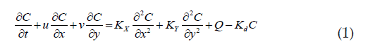
The latter which reproduces the behaviour of the pollutants in the study area, where is concentration at point M and time t in (ug/m³ ), the diffusion coefficients in the x, y direction in (m²/s) and wind speeds in the direction, is masse flow (kg/s), the reaction coefficient and which represents the disappearance term.

Meshing of the Study Area

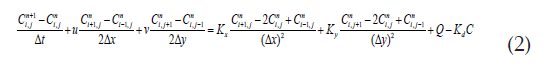
The prediction of the concentration of pollutant at a point of the domain can be obtained by first meshing the domain (Fig.6). More over by explicitly discretizing by finite difference the advection-diffusion equation in order to obtain the approximate value of the concentration in each time step and from the space. The discretization of the operators is done using the Taylor method. Either of the concentrations neighbouring the target concentration are used as input variables by the neural networks.

Figure 6: Mesh of the domain.

Standards and Air Quality

The standards governing air quality in Cameroon, defined by Law No. 96/12 of August 1996 on the framework law on environmental management of Decree No. 2011/2582/PM laying down the modalities of protection of the atmosphere specified in Table 1 (Eneo. 2018).

Tab.1: Standards and air quality in Cameroon

Results and Discussion

Performance of the GA-ANN Coupling

The evaluation of the performance of a model is done thanks to certain indices in particular the Mean Square Error (MSE), and the squared correlation coefficient (R²). A model is excellent when the squared error times towards zero, the coefficient of determination tends towards one. The Mean Square Error (MSE) is to evaluate the Deep Multi-output Long-Term Memory model. Anastasia used the squared correlation coefficient (R²) to evaluate artificial neural networks using a multilayer perceptron, which revealed that this model with a good performance in prediction (Anastasia, et al., 2011; Musy, et al., 1991).

The quality of this neural network model is evaluated on the basis of a test and training data set. This evaluation is presented by the Fig. 7. we have the vast majority of concentrations close to the fitting line to Y=X with a squared correlation coefficient R² is about 0.88 for the test case and R² is about 0.99 for the learned case which illustrates a fairly good performance of ANN in the test data, as the also shown in their work (Rongxiao, et al., 2018). The curve presents the root Mean Square Error (MSE); it is observed that the latter decrease with the number of iteration, and the best is about 0. 0044 (Fig. 8).

Figure 7: ANN prediction results on learning and testing. Note: Training- () Concentration; () Fit; () y=x; Test-() Concentration; () Fit; () y=x.

Figure 8: The Mean Square Error (MSE) of the Artificial Neural Network (ANN). Note: () Train; () Validation; () Test; () Best.

The fitness function curve evaluates the performance of two algorithms which are PSO and GA (Fig. 9). It is observed that the fitness function of GA and PSO grow almost similarly, however GA has the better fitness function from the beginning of the iteration to the end than the swarm per particle optimization. Bin had similar results comparing the particle swarm optimization method and the particle swarm optimization-simulated annealing hybridization (Bin, et al., 2018).

Figure 9: The fitness function of each algorithm at each iteration. Note: () ANN-PSO; () ANN-GA.

The validation of the GA-ANN coupling by comparing its results with the direct monitoring model, the CFD model and the Gaussian model (Fig.10). These results show that compared to the concentration evolution curve of the direct monitoring model, the GA-ANN coupling underestimates some concentration values with time.

Figure 10: Comparison of the GA-ANN coupling with other models. Note: () Monitoring; () GA-ANN ;() CFD model; () Gaussian model.

However, it can be seen that the GA-ANN coupling is more accurate than the CFD and Gaussian model.

Evaluation of Pollutant Emissions During 5 Years

The measurements of the emissions of the pollutants coming from the groups in operation were carried out in real time, between January 2017 and December 2021. To do this, they were carried out for the most part in the machine room by placing the test rod inside the exhaust pipes coming from the combustion chambers of the groups.

The curves respectively show the emissions of CO, NO₂, SO₂ and PM₁₀ between January 2017 and December 2021. Fig. 11 shows a peak in CO emissions of E=1.8 × 10⁶ kg in March 2018. (Fig.12) shows a peak in NO₂ emissions of E=9 × 10⁸ kg in August 2021. Fig. 13 shows a peak in SO₂ emissions of E=1.9 × 10⁸ kg in February 2019. Fig. 14 shows a peak in PM₁₀ emissions of E=4.5 × 10⁶ kg in March 2019. All these different emission peaks reflect a high level of activity of the thermal power plant of Yassa during these different months.

Figure 11: Monthly evolution of CO emission. Note: () 2017; () 2018; () 2019; () 2020; () 2021.

Figure 12: CMonthly evolution of NO₂ emission. Note: () Monitoring; () GA-ANN ;() CFD model; () Gaussian model.

Figure 13: CMonthly evolution of SO₂ emission. Note: () Monitoring; () GA-ANN ;() CFD model; () Gaussian model

Figure 14: CMonthly evolution of PM₁₀ emission. Note: () Monitoring; () GA-ANN ;() CFD model; () Gaussian model.

Evolution of Pollutants in Space and Time

In May 2021 the atmosphere is stable, the majority of these pollutants are inert and do not undergo chemical transformation on a local scale, therefore the reaction coefficient Kd=0; the diffusion coefficients are KY=10^-5 m/s and KZ=10^-5 m/s; the wind speeds are U=0 Km/h and V=10 Km/h; masse flow is QS= 0.29 kg/s. During this period, thanks to these field data, we were able to obtain the concentration distribution provided by the micro-sensors located at an altitude of 75 m in real time in May 2021 and the distribution curve provided by the GA-ANN coupling (Figs.15 and 16). It can be seen that the concentration distribution from the monitoring is almost similar to that from the GA-ANN coupling.

Figure 15: Concentration distribution provided by real-time micro-sensors in May 2021. Note: KY=10-5; KZ=10-5; U=0; V=18; QS=O.29.

Figure 16: Concentration distribution from the GA-ANN coupling. Note: KY=10-5; KZ=10-5; U=0; V=18; QS=O.29.

In March 2019 the atmosphere is unstable, the majority of these pollutants are inert and do not undergo chemical transformation on a local scale, therefore the reaction coefficient Kd=0; the diffusion coefficients are KY=10^-5 m/s and KZ=10^-5 m/s; the wind speeds are U=0 Km/h and V=18 Km/h; and masse flow is QS=0.29 kg/s During this period, thanks to these field data, we were able to obtain the concentration distribution provided by the micro- sensors located at an altitude of 75 m in real time in March 2019 and the distribution curve provided by the GA-ANN coupling Figs.17 and 18. It can be seen that the concentration distribution from the monitoring is almost similar to that from the GA-ANN coupling.

Figure 17: Concentration distribution provided by real-time micro- sensors in March 2019. Note: KY=10-5; KZ=10-5; U=0; V=18; QS=O.29.

Figure 18: Concentration distribution from the GA-ANN coupling. Note: KY=10-5; KZ=10-5; U=0; V=18; QS=O.29.

Pollutant Dispersion by Source Flow and Wind Regimes

The curves from the monitoring and GA-ANN coupling show the evolution of the concentration of Carbon Monoxide (CO), Sulphur Dioxide (SO₂), Nitrogen Dioxide (NO₂) and Particulate Matter (PM₁₀) in the south-westerly direction where the winds are stronger Figs.19-21. It can be seen on each of the figures that for a value of flow taken from the database, the evolution curve of the observed pollutant concentration and the GA-ANN coupling is shown. It can also be seen on the different figures that the concentrations from the GA-ANN coupling, although different from those from the monitoring in some areas far from the source, are approximately equal near the source. It can be deduced that in some areas far from the source, the GA-ANN coupling underestimates some concentration values, and close to the source this model gives accurate concentration values.

Figure 19: Evolution of pollutant concentration in space. Note: () GA-ANN; () Monitoring.

Figure 20: Evolution of pollutant concentration in space. Note: () GA-ANN; () Monitoring.

Figure 21: Evolution of pollutant concentration in space (Q=0.2). Note: () GA-ANN; () Monitoring.

The curves from the monitoring and GA-ANN coupling show the evolution of the concentration of Carbon Monoxide (CO), Sulphur Dioxide (SO₂), Nitrogen Dioxide (NO₂) and Particulate Matter (PM₁₀) in the south-western direction where the winds are stronger Figs.22-24. It can be seen on each of the figures that for a value of the velocity taken from the database, we have the evolution curve of the concentration of the observed pollutants and the GA-ANN coupling. It can also be seen on the different figures that the concentrations from the GA-ANN coupling, although different from those from the monitoring in some areas far from the source, are approximately equal near the source. It can be deduced that at some locations far from the source, the GA-ANN coupling underestimates some concentration values, and close to the source this model gives accurate concentration values.

Figure 22: Evolution of pollutant concentration in space. Note: () GA-ANN; () Monitoring.

Figure 23: Evolution of pollutant concentration in space. Note: () GA-ANN; () Monitoring.

Figure 24: Evolution of pollutant concentration in space (Monitoring). Note: () GA-ANN; () Monitoring.

Conclusion

This paper proposes a new atmospheric dispersion model for air quality forecasting. In this work, the coupling of genetic algorithm and neural networks was developed and evaluated by comparing it to monitoring tools and other models. Genetic algorithms were used as objective function optimisation tools. Meteorological data, source data and the advection-diffusion term were used as inputs to the neural networks to estimate the concentration of Carbon Monoxide (CO), Nitrogen Dioxide (NO₂), Sulphur Dioxide (SO₂), Particulate Matter (PM₁₀). These results showed that the GA-ANN coupling, although underestimating the concentrations at some points far from the pollution source, is a very accurate and fast prediction model near the source. The results also show that the GA-ANN coupling is more accurate than the CFD and Gaussian model.

Author’s Contribution

All authors contributed equally to this work.

Acknowledgements

This work was supported by the University of Yaoundé I-Cameroon. The work carried out in the framework of this draft paper was also supported by the laboratory of the Ecole Normale Supérieure of Yaoundé under the supervision of Professor Beguide Bonoma (Head of the physics departement of this school); by the energy and thermal enegineering laboratory of the Ecole National Polytechnique of Maroua under the supervision of professor Nsouandele Jean-Luc. The data was taken by the company in charge of electricity in Cameroon (Eneo) and permission was grasynted by its director general, in one of its production Yassa-Dibamba thermal power plant). The work of analysis, interpretaion, results and writing was done in the Energy, Electrical and Electronic System laboratory, Research and training Unit of physics, University of Yaounde I-Cameroon, during 9 months.

Funding

This work was not financially supported.

Declaration of Competing Interest

The authors declare that yhey have no known competing financial interests or personal relationships that could have appeared to influence the work reported in this paper.

Provide the Data Availability Statement

The data used to support the conclusions of this study are available on the zonodo accredited website from the link below.

• Goune AC, Seutche J C and Nsouandele J L. 2022. Database of thermal power plant of YASSA-DIBAMBA CAMEROUN (2017-2018-2019-2020-2021) . Zenodo.

References

1. Liu M, Bi J and Ma Z. 2017.Visibility-based PM2.5 concentrations in China: 1957-1964 and 1973-2014. Environ Sci Technol. 51(22): 13161-13169.

   [Crossref] [Google Scholar][PubMed]

2. Apte JS, Marshall JD, Cohen AJ and Brauer M. 2015.Addressing global mortality from ambient PM2.5. Environ. Sci. Technol. 49(13): 8057–8066.

   [Crossref] [Google Scholar][PubMed]

3. Lin B and Zhu J. 2018. Changes in urban air quality during urbanization in China. J Clean Prod. 188(4):312-321.

   [Crossref] [Google Scholar]

4. Li N, Chen JP, Tsai CI. 2017. Potential impacts of electric vehicles on air quality in Taiwan. Sci Total Environ. 566(5):919-928.

   [Crossref] [Google Scholar][PubMed]

5. Andre JC and Royal JF. 1999. Short-term climate fluctuations and the interpretation of recent observations in terms of the greenhouse effect (Short-term climatic fluctuations and the interprétation of récent observations in terms of greenhouse effect). Series IIA-Earth Planet. Sci. 328 (4): 261–272.

   [Crossref] [Google Scholar]

6. Li H, You S, Zhang H, Zheng W, Lee WL, Ye T and Zou L. 2018. Analyzing the impact of heating emissions on air quality index based on principal component regression. J Clean Prod .171(1) 1577-1592.

   [Crossref] [Google Scholar]

7. Konga mopoum Nk. 2005. Influence of the canopy and the clearing regime on the growth of young cocoa trees (theobroma cacao.I) in the mbalmayo forest reserve. Yaounde: University of Yaounde I.
8. Federal Ministry for Economic Cooperation and Development. 2013. Pilot study on surface and groundwater pollution in yaounde and its impact on the health of local populations (EPESS). Yaounde : National statistical institute.
9. Roemer W, Hoek G, Brunekreef B, Clench-aas J, Forsberg B, Pekkanen J and Schutz A. 2000. PM10 elemental composition and acute respiratory health effects in european children (PEACE project). Eur Respir J. 15(5): 553-559.

   [Crossref] [Google Scholar][PubMed]

10. Middleton N, Yiallouros P, Kleanthous S, Kolokotroni O, Schwartz J, Dockery DW, Demokritou P and Koutrakis P. 2008. A 10-year time series analysis of respiratory and cardiovascular morbidity in Nicosia, Cyprus: the effect of short-term changes in air pollution and dust storms. Environmental Health. 7(3): 39.

    [Crossref] [Google Scholar][PubMed]

11. Lemiere B, Seguin JJ, Guern le C, Gyonnet D and Baranger P. 2001. Guidance on the behaviour of pollutants in soil and groundwater: Application in the context of a detailed risk assessment for water resources.
12. Pascal MI, Debertini AV and François MK.2011. Case study of pollutants concentration sensitivity to meteorological fields and land use parameters over douala (cameroon) using aermod dispersion model. Atmosphere. 2(4): 715-741.

    [Crossref] [Google Scholar]

13. Ministry of Sustainable Development, the environment and the fight against climate change. 2017. Preparation and realization of a modeling of the dispersion of the atmospheric emissions of the mining project.
14. Pournazeri S, Tan S, Schulte N, Jing Q and Venkatram A. 2014. A computationally efficient model for estimating background concentrations of NOx, NO2, and O3. Environ Model Softw. 52(6):19-37.

    [Crossref] [Google Scholar]

15. YangY and ChristakosG.2015. Spatiotemporal characterization of ambient pm2.5 concentrations in shandong province (china). Environ Sci Technol. 22(49):13431-13438.

    [Crossref] [Google Scholar][PubMed]

16. Corani G and Scanagatta M. 2016. Air pollution prediction via multi-label classification. Environ Model Softw. 80 (6):259-264.

    [Crossref] [Google Scholar]

17. Wakeel M, Yang S, Chen B, Hayat T, Alsaedi A and Ahmad B. 2017. Network perspective of embodied PM2. 5-A case study. J Clean Prod.142(4):3322-3331.

    [Crossref][Google Scholar]

18. Van Fan Y, Perry S, Klemes JJ and Lee CT. 2018. A review on air emissions assessment: Transportation. J Clean Prod. 194(3): 673-684.

    [Crossref] [Google Scholar]

19. Yang G, Huang J and Li X. 2018. Mining sequential patterns of PM2.5 pollution in three zones in China. J Clean Prod. 170(4):388-398.

    [Crossref] [Google Scholar][PubMed]

20. Hanna SR, Briggs GA, Hosker RP and Smith JS. 1982. Handbook on atmospheric diffusion. Washington, United States: Office of Health and Environmental Research.
21. Bieringer P E, Rodriguez LM, Vandenberghe F, Hurst JG, Bieberbachb G, Sykes I, Hannan JR, Zaragoza J and Fry RN. 2015. Automated source term and wind parameter estimation for atmospheric transport and dispersion applications. Atmos.EnvironB.122 (1):206-219.

    [Crossref] [Google Scholar]

22. Florian V. 2011. Modeling atmospheric dispersion in the presence of complex obstacles: application to the study of industrial sites. Lyon: the University of Lyon.
23. Pierre L, Frederic H, Laurent A, Anne J.2016. Atmospheric dispersion modeling using artificial neural network based cellular automata. Environ Model Softw. 85(6):56-69.

    [Crossref] [Google Scholar]

24. Sihang Q, Bin C, Rongxia W, Zhengqiu Z, Yuan W and Xiaogang Q. 2018. Atmospheric dispersion prediction and source estimation of hazardous gas using artificial neural network, particle swarm optimization and expectation maximization. Atmos Environ. 178(4):158-163.

    [Crossref] [Google Scholar]

25. Bin C ,Rongxiao W, Sihang Q, Liang M, Zhengqiu Z, Yiping W and Xiaogang Q.2018. Hazardous source estimation using an artificial neural network, particle swarm optimization and a simulated annealing algorithm. Atmosphere. 9(4):119.

    [Crossref] [Google Scholar]

26. Rongxiao W, Bin C, Yiduo W, Zhengqiu Z, Liang M and Xiaogang Q.2018. The air contaminant dispersion prediction by the integration of the neural network and aermod system. International Workshop on Safety and Resilience. 11: 1-5.

    [Crossref] [Google Scholar]

27. Juan SRM, Thierno D, Bernard C, Marc A and Karim L.2022. Vapor intrusion in buildings: Development of semi-empirical models including lateral separation between the building and the pollution source. Building simulation.2031-2049.

    [Crossref] [Google Scholar]

28. Seutche JC, Nsouandélé JL, Njingti-Nfor, Tamba JG and Bonoma B.2019. Geographical mapping and modelling of noise pollution from industrial motors: a case study of the mbalmayo thermal power plant in cameroon. Environ Monit Assess. 191(4):765.

    [Crossref] [Google Scholar][PubMed]

29. Seutche NJC. 2012. Impact of heavy fuel oil combustion on the environment in the oyom-abang thermal power plant. Yaoundé: University of Yaoundé 1.
30. Robbins H and Monro S. 1951. A stochastic approximation method. Ann Math Stat. 22(6): 400-407.

    [Crossref] [Google Scholar]

31. Ostad-Ali-Askari, Shayannejad and Ghorbanizadeh-Kharazi H. 2017. Artificial neural network for modelling nitrate pollution of groundwater in marginal area of zayandeh-rood River, isfahan, Iran. Journal of Civil Engineering. 7(2):134-140.

    [Crossref] [Google Scholar]

32. Pierre L. 2013. Atmospheric dispersion modelling on an industrial site using a combination of cellular automata and neural networks.
33. Bellatreche L and Boukhalfa K. 2005. Fragmentation in data warehouses: an approach based on genetic algorithms. New information technology review in EDA.
34. Thomas V and Murat Y.2001. Presentation of genetic algorithms and their applications in economics. ResearchGate.
35. Hanaa H, Youssfi Ek and Mariam E. 2013. Hybridization of metaheuristic algorithms in global optimization and their applications. Rabat: Mohammadia School of Engineering.
36. Eneo. 2018. Eneo annual report. Yaoundé.
37. Anastasia KP, Spyrindon K, Savvas K and Pavlos AK.2011. Forecasting hourly PM10    concentration in Cyprus through artificial neural networks and multiple regression models: implications to local environmental management. Environ Sci Pollut Res.18(5):316–327.

    [Crossref] [Google Scholar][PubMed]

38. Musy A and Soutter M. 1991. Soil physics. Presses polytechniques et universitaires romandes.