
ISSN (0970-2083)
ISSN (0970-2083)
Piyali Majumder*
Associate Fellow, National Council of Applied Economic Research (NCAER), New Delhi, India
Received: 20-Sep-2023, Manuscript No. ICP-23-114404; Editor assigned: 25-Sep-2023, PreQC No. ICP-23-114404 (PQ); Reviewed: 11-Oct-2023, QC No. ICP-23-114404; Revised: 18-Oct-2023, Manuscript No: ICP-23-114404 (A); Published: 25-Oct-2023, DOI: 10.4172/0970-2083.005
Citation: Majumder P. Development of Organized Manufacturing Sector Across Indian Atates-A Spatial Approach. J Ind Pollut Control. 2023;39:005.
Copyright: © 2023 Majumder P. This is an open-access article distributed under the terms of the Creative Commons Attribution License, which permits unrestricted use, distribution, and reproduction in any medium, provided the original author and source are credited.
Visit for more related articles at Journal of Industrial Pollution Control
The paper examines the nature and pattern of development of the Indian organized manufacturing industries across Indian states using the Annual Survey of Industries (ASI) plant-level data. Four different indices of industrial concentration have been used to estimate the degree of agglomeration of industries. It has been observed that states with a large industrial base are also the hub of some of the highly polluting industries. The degree of industrial agglomeration has been observed to be higher in the case of polluting industries as opposed to non-polluting industries in the year 2013-14. The degree of agglomeration economies of the industry has been observed to be affected by the spillover effect from the adjacent regions. While examining the pattern of spatial concentration of industries over time, the paper concludes that during the period of the analysis 2000-01 to 2013-14, the polluting industries have shown some dispersion both across states (captured by the LQ index) as well as in terms of plant level concentration within-in the same industry.
Organised manufacturing sector, Spatial development, Agglomeration economies.
The spatial disparity in the distribution of economic activities is a widespread phenomenon all over the world. Silicon Valley of California, the Diamond District of Manhattan, automobile manufacturing clusters of Detroit, the IT hub of Bangalore, small carpet-making clusters of Agra, and the Drugs and Pharmaceuticals clusters of Ahmadabad are examples of some of the famous manufacturing clusters across the world. Why do firms prefer to locate in certain regions? How the clusters are formed and how do they evolve over time? These are some of the questions that entail deeper economic analysis and have received substantive attention, both from academic researchers as well as policy-makers.
The tendency of plants to co-locate near each other within a few regions is driven by several distinct factors. While some firms may be concentrated in a region due to the availability of specific natural resources or proximity to consumer markets; sometimes concentration may be even triggered by some historical events. It has been observed that plants tend to concentrate near the already existing clusters thereby further reinforcing the industrial agglomeration. The location-specific benefits arising from the co-location of plants and interdependences of economic agents within the same industry are termed localisation economies. In contrast to this, any other locational benefits external to the industry are termed urbanisation economies. Ciccone broadly identified three types of benefits that a plant may get by locating near other plants, viz; availability of a specialised pool of labour, buyer-supplier linkages and spillover of technological know-how (Ciccone, et al., 1993). There exists extensive literature that has examined the scope of localisation economies and urbanisation economies in the context of developed nations (Rosenthal, et al., 2004). While analyzing the scope of agglomeration economies, it is also pertinent to examine the nature of the agglomeration i.e., which type of industry is concentrated across space? Studies in the context of developed countries have empirically shown that the degree of agglomeration and the underlying forces driving the concentration largely differ across industries (Devereux, et al., 2004). However, analysing the nature of industrial agglomeration and estimating the degree of concentration of industries across space is an emerging literature in the Indian context (Lall, et al., 2004). The present paper attempts to estimate the degree of industrial agglomeration in the Indian organised manufacturing sector at a disaggregated level of industrial classification (at the four-digit level NIC2008 classification) for the year 2013-14 using the information on plant-level employment across Indian states. The paper also analyses the nature of this agglomeration by distinguishing between polluting vs. non-polluting industries. Moreover, the paper also compares the evolution pattern of industrial agglomeration over the period 2000-01 to 2013-14.
The paper uses four different indices of industrial concentration to analyse the extent and nature of the spatial distribution of manufacturing industries across Indian states over time. It has been observed that states with a large industrial base are also the hub of some of the highly polluting industries. The degree of industrial agglomeration has been observed to be higher in the case of polluting industries as opposed to non-polluting industries in the year 2013-14. The extent of agglomeration economies in industry has been observed to be affected by the spillover effect from adjacent regions. While examining the pattern of spatial concentration of industries over time, the paper concludes that during the period of the analysis 2000-01 to 2013-14, the polluting industries have shown some dispersion both across states (captured by the LQ index) as well as in terms of within-in industry concentration (captured by the EG index). Compared to the scenario in 2000-01, it is true that these industries have dispersed over time, but the environmental concern associated with the concentration of polluting industries, remains as they still appear to be highly agglomerated in the year 2013-14. Moreover, they also constitute a bulk of the share of total manufacturing output in some of the peripheral states of India.
The first section of the paper gives a brief review of the theories explaining the mechanism behind industrial agglomeration and their evolution over time. It also discusses several indices that have been constructed to the measure the degree of industrial agglomeration. The second section of the paper elaborates the nature and different features of industrial agglomeration in Indian organised manufacturing sector. The third section explains the pattern of evolution of industrial agglomeration over time across Indian states and industries. The fourth section concludes the paper with a discussion on the observed features of agglomeration and its implication in the Indian organised manufacturing sector.
Evolution Theories of Industrial Agglomeration
The study of unevenness in the spatial distribution of economic activities can be traced back into the early works of Cingano monocentric city model and central place theory and Alonso and urban system theory (Cingano, et al., 2004; Alonso, et al., 2004). Combes, urban system theory assumed that there exists a Central Business District (CBD) within a country where economic activities and consumers tend to concentrate(Combes, et al., 2015). The availability of infrastructural amenities, presence of large consumer markets, port facilities; and other urban amenities create some externalities which further draws in new investors, thereby reinforcing the clustering process within the CBD. These theories were criticised later, as they did not analyze the underlying mechanism behind the formation of CBD (Das, et al., 2015). Moreover, these theories were primarily focused on analyzing the efficient allocation of space for production activities within the CBD and neglected the relevance of periphery (or non-urban space) within a country.
The location theories of firm and Datta explained the role of transport costs in determining the location of manufacturing activities in urban areas as opposed to non-urban space (Datta, et al., 2011). They analysed the location decision of a producer in presence of a trade-off between transport costs and market demand, under a perfectly competitive market structure. However, as indicated in the urban system theories, clustering of economic activities entails presence of some form of increasing return to scale or economies of scale. Modelling of increasing return to scale implies presence of imperfectly competitive market structure. Under the perfect competition assumption, these theories have also failed to model the underlying economies of scale, arising from the interaction between economic agents and other location-specific attributes that influences the location decision of a producer.
Modelling of imperfect competition at the firm level can be traced back into the trade theory literature. (Krugman,1991) in a general equilibrium framework showed that how presence of economies of scale, transport costs and differential market size endogenously determines firm’s decision to concentrate its production activity in a particular region of a country; giving rise to core-periphery dichotomy pattern of development. Using simulation techniques, he showed that the producer’s propensity to agglomerate or disperse is dependent on some critical threshold values of economies of scale, transport costs and market demand for the manufactured goods. The relevance of geographical attributes in shaping the development of economic activities across space, re-gained its importance with this modelling strategy; also marked as the New-Economic Geography (NEG) era. While internal economies of scale, as modelled by (Krugman, 1991) is an important factor in driving agglomeration of industries, external economies of scale also reinforce the concentration of industries.
Firms within the same industry or related industries may co-locate near each other to enjoy a cost advantage in terms of easy availability of industry-specific factors of production (labour market pooling advantage) or diffusion of technology/knowledge or availability of specialised intermediate inputs across firms. In contrast to this, economies arising from the co-location of related or unrelated industries, availability of transport amenities, accessibility to large consumer markets or any other location-specific benefit outside own-industry is termed as urbanisation economies. Both urbanisation economies and localisation economies have been observed to drive the concentration of manufacturing activities. These economies act as centripetal forces to reinforce the concentration process further.
Indices for Empirical Estimation of Industrial Agglomeration Economies
estimate the degree of industrial agglomeration across spatial units. It has been observed that the degree of agglomeration varies across different levels of spatial aggregation (the degree of agglomeration in the same industry may vary when measures at the district-level/county level vs. at the state-level), as well as different levels of industrial aggregation (agglomeration of industry, measured at the two-digit level differs from the agglomeration measured at the four-digit level). The existing indices can be broadly categorized into two categories-the discrete indices of industrial agglomeration where spatial units are discrete Dougherty and continuous indices where spatial units are considered to be continuous (Dougherty, et al., 2011). The continuous indices are distance-based measures where kernel density function is estimated using the distance between pair of plants. This requires accurate location of a plant, which is often unavailable. Moreover, the theoretical foundation of these indices is emerging and beyond the scope of the present study.
The discrete indices can be further grouped into two broad categories viz; the raw measures of geographical concentration and the plant-based measures of industrial agglomeration. The raw measures of geographic concentration of an industry viz; Hoover’s Location quotient 1936 and Krugman’s spatial Gini coefficient 1991 captures the disparity in the distribution of regional employment (or output) in an industry relative to the regional-distribution of overall employment (or employment) in the country. One of the major criticisms of raw measure of industrial agglomeration, these indices did not consider the within-industry plant structure which may have driven the degree of concentration of an industry. Suppose we have two industries, industry 1 and industry 2. Industry 1 is characterized by many plants all concentrated in one specific region whereas industry 2 is characterized by a single plant. Despite having dissimilar within-industry structures both the industries will show similar Gini coefficient. In industry 1 concentration may be driven by the region–specific external economies; however, in industry 2, concentration is solely driven by the plant structure within the industry i.e. the entire production is concentrated within a plant. This feature makes these indices irrelevant for cross-industry comparisons of the degree of agglomeration.
While constructing an index to measure the degree of spatial concentration of an industry, the main challenge has been to incorporate the randomness involved in the agglomeration process i.e., some industries may be agglomerated spatially just by chance. Ellison proposed a location choice model for an industry where the probability of choosing a location by an industry is dependent on the natural advantages of that geographic area (availability of raw materials, water and electricity supply, large consumer markets, network of inter-industry linkages) and externalities arising from the co-location of plants within the industry (Ellison, et al., 1997). They defined agglomeration as the geographic concentration of an industry in excess of the plant-level concentration within the industry. This is also known as industrial localisation index.
Similar to Ellison (MS) formulated another index to measure the degree of industrial agglomeration. Both the indices measure geographic concentration of an industry after controlling the effect of within industry concentration. However, while calculating the degree of agglomeration of an industry, the two indices differ in the way they give weightage to the concentration of overall economic activity in a region. For example, if an industry is located in a highly industrialised area, then MS index takes on high value whereas if an industry is located in a less industrialized area, then the value of the index is lower. In case of EG index there is no such distinction made and the value is same in both the cases.
The Gini, Location Quotient, EG or MS indices captures the concentration of an industry as they quantify the variability in employment (or output) of an industry across spatial units relative to the national average. Arbia argued that these indices did not capture the actual geographical location of a production unit with respect to the other adjacent regions i.e. the spatial correlation between the economic activities of region i and the economic activities of neighbouring regions (Arbia, et al., 2001). Moreover, using the spatial unit data defined by boundaries, the degree of industrial concentration is calculated within a pre-defined spatial unit. In the spatial econometrics literature this is also termed as modified area unit problem (Anselin, et al., 1988). To account for both the neighbourhood effect as well as to correct the MAUP, indices of industrial concentration i.e. Gini, Location Quotient, EG or MS are weighed by using the row-standardized spatial weight matrix. The spatial weights matrix captures the spatial dependence between the units of observations. The weights can be generated using the number of neighbours (contiguity-based) or the distance between the adjacent observations (distance-based). The spatially weighted indices capture the degree of ‘spatial’ agglomeration of an industry in true sense.
Most of the studies analysing the pattern of industrial agglomeration across different levels of spatial aggregation has been a focus for many researchers since past few decades in both the developed as well as developing countries (Deichmann, et al., 2008). The literature has been emerging in the context of developing countries especially in India.
Spatial Development of Manufacturing Industries-Experience of India
While analysing the pattern of regional unevenness across Indian states, indicated that the colonial legacy of India under British rule inculcated a core-periphery dichotomy pattern in the development process of manufacturing industries. Britishers guided by their own economic incentives, channelized investment only for the development of the port towns of Calcutta, Bombay and Madras in terms of the availability of infrastructure, and other amenities. However, in the post-independence era, liberalization policies of India in 1991 marked the end of industrial licensing regime and industries were free to locate according to their profitability.
Industries usually tend to locate to places characterised by availability of raw materials required in the production process and easy accessibility to consumer markets where it can cater its products. Over time freight policies have been revised to negate the locational advantages of proximity with raw materials i.e. industries located at any place of the country will get some of the critical inputs like coal, cement, iron ore, aluminium etc required for the development of industries at the same prices as that of the industries located in mineral-rich states. However, these policies facilitated agglomeration of industries in states characterised by large consumer markets as opposed to industrially backward but resource-rich states such as Bihar, Madhya Pradesh and Orissa, thereby aggravating the regional imbalance further. Other locational policies like provision of adequate infrastructural amenities across states play a significant role in shaping the spatial development process of industries. Infrastructural facilities include availability of power and water supply, telecommunication, banking services, transport-related infrastructures like roads and railway connectivity etc. Transport cost is a significant factor in determining the location of an industrial unit. To ensure better connectivity, across states over the period, Government of India has recommended the establishment of industrial corridors, improvement of connectivity of national highways (Golden Quadrilateral), development of rural roads under the Pradhan Mantri Gram Sadak Yojana (PMGSY, 2000) scheme (Amirapu,et al., 2019).
The development of small-scale traditional artisan industrial clusters significantly minimised the rural-urban divergence in the industrial development process within Indian states. However, inter-state disparity in the development of the manufacturing industries has remained an important area of concern in the Indian economy. Presently, states like Gujarat, Andhra Pradesh, Maharashtra, Tamil Nadu and Punjab have emerged as the hub of diversified industrial activities in India at the expense of the states like Assam, Manipur, Nagaland and Jammu and Kashmir, Himachal Pradesh which remained industrially backward (Chakravorty,et al., 2003). It has been empirically observed that the presence of intra-industry spillovers, inter-industry linkages, availability of infrastructural facilities (urban amenities) like availability of proper transport infrastructure ensuring easy accessibility to input and output markets, electricity, water etc. and government policies are some of the driving forces (centripetal forces) behind reinforcing agglomeration of industries in Indian organised manufacturing sector (Mukim, et al., 2014). The high-tech industries like manufacturing of machinery equipment and manufacturing of electronics and computer equipments are found to be concentrated mostly in urban areas as opposed to the low-end manufacturing industries like food and beverages, leather processing and tobacco industries. The high-tech innovative industries have greater ability to pay high wages and land rents prevailing in densely populated urban areas compared to the low-end manufacturing industries. The externalities arising from the availability of infrastructural facilities, large consumer markets, presence of diversified industrial base or cross-industry economies, were found to have a positive and significant impact on the productivity of these high-tech industries (Lall, et al., 2005).
Low-end manufacturing industries like food and beverages, leather processing and tobacco industries were mostly found to benefit from within-industry economies i.e. industry-specific labour pool, technical know-how and are located in rural areas of the country (Ghani, et al., 2012). While analysing the within-industry agglomeration pattern of the manufacturing sector found that within the same industry there is a high spatial corelation between formal and informal sector firms. She observed that informal firms are engaged in catering the demand of labour and raw materials demand inside the same industry. In her analysis, she has emphasized the channel of buyer-supplier linkage as one of the significant factors in driving the higher degree spatial correlation between formal and informal firms within the same industry.
While analysing the evolution of industrial agglomeration over time it has been observed that the organised firms, located in urban areas are moving towards rural or peri-urban areas i.e., the share of employment of organised firms in urban areas show a declining trend whereas their share has been rising in the rural areas/peri-urban areas. In contrast, unorganised manufacturing firms registered a high employment growth in the urban areas it concluded that scale economies available in urban areas are more important for the small firms under unorganised sectors compare to the larger firms under organised sector. The manufacturing of non-metallic mineral products, Tobacco products and Food products and beverages are some of the least urbanised industry with less than 30% employment in urban areas. However, industries like manufacturing of machinery and equipment, office, accounting and computing machinery experienced an increase in their urban employment share in the year 2000 compared to the employment share. The observed pattern of evolution of manufacturing industries has been termed as ruralisation of the organised manufacturing sector.
The overall expansion of manufacturing activities in India has raised serious concern about the environmental problems associated with it. Industrial emissions have significantly led to the deterioration of the environmental quality. It has significantly aggravated the concentration of pollutants like NO2 and SO2 in the air (Fernandes, et al., 2012). While estimating the pollution-load of the Indian organised manufacturing sector using the Industrial Pollution Projection System (IPPS) by World Bank, it has been observed that with the increase in industrial output, industrial pollution load also shows an increasing trend. Based on the pollution load of industries the study identified top ten polluting industries of India viz manufacturing of vegetable and animal oils, sugar, drugs and pharmaceuticals, cement, fabricated metal products, fertilizer and nitrogen compounds, basic and other non-ferrous metals, coke and refined petroleum, rubber and tyres. However, there is no study on analysing the pattern and degree of agglomeration of polluting industries in India. A study analysing the pattern and degree of spatial concentration of polluting industries would assist to identify the polluted regions across the country. This in turn will facilitate formulation of policies (especially area-based environmental management policies by regulating the location of these industries in already polluted areas) to mitigate the environment problems arising from the geographic concentration of manufacturing activities; especially that of the polluting industries.
Several attempts have been taken by the CPCB and the SPCBs to prepare a comprehensive environmental mapping for the location of industries (‘Zoning Atlas for siting industries’) across all districts. This mapping scheme engrafts both economic factors such as availability of raw materials, water and power supply, factor inputs like labor as well as the environmental factors (i.e. air, water quality of a location) that are required to be considered before a new industry is allowed to set up (CPCB 2010). This helps the entrepreneurs to find a suitable location which is economically and environmentally viable for the sustenance of their production process. Moreover, CPCB has also initiated the Environmental Impact Assessment Programme, under which entrepreneurs are issued environmental clearance certificates after assessing the potential environmental risk associated with their projects. However, the compliance with the industry-specific emission standards is monitored by the State Pollution Control Board (SPCB) and the degree of enforcement of environmental laws varies across states.
The present paper of the study attempts to fill the gap in the literature by examining the degree of agglomeration of organised manufacturing industries across Indian states, especially featuring out the concentration of polluting industries and their evolution pattern over time. Unlike the previous studies in Indian context, the present paper analyses the degree of industrial agglomeration at a finer level of industrial classification (four-digit industries), thereby reflecting the polluting nature of industries. For example, industries like leather tanneries and manufacturing of leather products which differ in their polluting nature can be distinguished at a four-digit level of industrial classification whereas at the two-digit level they are clubbed together under manufacturing of leather.
Nature of Industrial Agglomeration in Indian Organised Manufacturing Sector
Data: The spatial concentration of the organized Indian manufacturing industries has been estimated based on the Annual Survey of Industries (ASI) factory-level database, one of the primary sources of industrial statistics in India. It covers all manufacturing factories registered under the sections of Factories Act of 1948. A factory is the primary unit of enumeration in the survey process. It is defined as any manufacturing unit with an employment of 10 or more workers using power and those with 20 or workers not using power. Other than solely manufacturing units, all electricity undertakings, engaged in transmission, generation and distribution of electricity. Moreover, some of the units engaged in services like repairing of motor vehicles, water supply, and cold storage also comes under the purview of the ASI survey. However, in this study our entire analysis is strictly restricted to units solely engaged in the manufacturing process.
Data: The spatial concentration of the organized Indian manufacturing industries has been estimated based on the Annual Survey of Industries (ASI) factory-level database, one of the primary sources of industrial statistics in India. It covers all manufacturing factories registered under the sections of Factories Act of 1948. A factory is the primary unit of enumeration in the survey process. It is defined as any manufacturing unit with an employment of 10 or more workers using power and those with 20 or workers not using power. Other than solely manufacturing units, all electricity undertakings, engaged in transmission, generation and distribution of electricity. Moreover, some of the units engaged in services like repairing of motor vehicles, water supply, and cold storage also comes under the purview of the ASI survey. However, in this study our entire analysis is strictly restricted to units solely engaged in the manufacturing process.
The sampling stratum of a manufacturing unit is defined by its geographical location, viz, state and district, industry group (at the 4-digit level of NIC) and sector. The multiplier weights are used to generate estimates at these four sub-sample levels i.e. state, district, industry group and sector. The availability of geographical location of a factory along with the other characteristics like output, raw materials (including types of fuel consumed), types of fixed assets used in the production process, workers employed in each unit, ownership structure and export share, makes this database ideal for analyzing the pattern and the underlying agglomerating/dispersing forces in driving the spatial development process of the organized manufacturing industries in India.
The survey covers all manufacturing units, registered under the Factories Act of 1948 across 29 states and 7 union territories except Arunachal Pradesh and Union territory of Lakshadweep. The spatial coverage of ASI has been updated along with the change in the state boundaries in India for example ASI 2012-13 rounds started reporting data on Telangana. However, in the present study while analyzing the time series data, to maintain parity, the data of Telangana and Andhra Pradesh has been clubbed together.
In the present paper of the study the spatial pattern of development of manufacturing industries across Indian states has been analyzed, based on the latest year published data i.e. ASI 2013-14 round. While analyzing the evolution of industrial concentration over time in Section 3.3, comparison has been done between the patterns of industrial concentration in 2013-14 vs. the pattern observed in the year 2000-01. In the year 2013-14, the industrial concentration has been estimated for all the 125 manufacturing industries as defined at the four-digit level of National Industrial Classification 2008 (NIC2008). These industries In the present paper of the study the spatial pattern of development of manufacturing industries across Indian states has been analyzed, based on the latest year published data i.e. ASI 2013-14 round. While analyzing the evolution of industrial concentration over time in Section 3.3, comparison has been done between the patterns of industrial concentration in 2013-14 vs. the pattern observed in the year 2000-01. In the year 2013-14, the industrial concentration has been estimated for all the 125 manufacturing industries as defined at the four-digit level of National Industrial Classification 2008 (NIC2008). These industries together represent 77% of the total output produced by all factories surveyed under ASI 2013-14 round. However, while assessing the evolution of industrial concentration, the degree of concentration of only 111 industries (defined at the four- digit level of NIC2008) could be compared between 2000-01 and 2013-14. The plant coverage across states has been reported from Table 1 below.
| State | Number of Plants( 2000-01) | Number of Plants( 2013-14) |
|---|---|---|
| Tamil Nadu | 23937 | 33645 |
| Andhra Pradesh* | 16487 | 28168 |
| Maharashtra | 23243 | 26652 |
| Gujarat | 21145 | 21551 |
| Uttar Pradesh | 12642 | 12846 |
| Punjab | 8424 | 11951 |
| Karnataka | 8328 | 10549 |
| Rajasthan | 5672 | 8365 |
| West Bengal | 7827 | 7943 |
| Kerala | 4914 | 6006 |
| Haryana | 5766 | 5857 |
| Madhya Pradesh | 3493 | 3636 |
| Delhi | 4242 | 3359 |
| Assam | 2085 | 3354 |
| Bihar | 1997 | 3142 |
| Uttaranchal | 933 | 2848 |
| Himachal Pradesh | 685 | 2686 |
| Orissa | 2029 | 2555 |
| Jharkhand | 1784 | 2412 |
| Chhattisgarh | 1645 | 2333 |
| Daman & Diu | 1548 | 1841 |
| Dadra & Nagar Haveli | 1143 | 1366 |
| Jammu & Kashmir | 391 | 911 |
| Pondicherry | 559 | 803 |
| Goa | 537 | 558 |
| Tripura | 244 | 522 |
| Chandigarh (U.T.) | 305 | 238 |
| Manipur | 65 | 138 |
| Nagaland | 156 | 126 |
| Meghalaya | 27 | 101 |
| Sikkim | Not Covered | 60 |
| Andaman & N. Island | 23 | 13 |
| Lakshadweep | Not Covered | Not Covered |
| Arunachal Pradesh | Not Covered | Not Covered |
| Mizoram | Not Covered | Not Covered |
Source: Author’s calculation based on ASI data
Note: *In the year 2013-14 data for Telangana and Andhra Pradesh were also clubbed together
Table 1. Spatial distribution of organised manufacturing plants
In this study, the estimation of industrial concentration of manufacturing industries defined at the four digit level of NIC-2008 is based on the plant-level employment data. It can be observed that there has been 26% growth in the number of plants over these 13 years. In the year 2013-14 there has been a substantive rise in the number plants employing more than 200 workers. This is driven by the revision of sampling coverage of ‘census sector plants’. The share of census sector plants in the year 2013-14 is 22% of the total plants covered under the survey as opposed to 10% in the year 2000-01. The coverage of plants across industries over time has been reported. Distribution of plant-level employment has been reported in Table 2.
| Year | Plants<=50workers | 50 <Plants<=200workers | Plants>200workers | Total Plants |
|---|---|---|---|---|
| 2000-01 | 148985 | 15972 | 6744 | 171701 |
| 2013-14 | 143915 | 25984 | 48158 | 218056 |
Source: Author’s calculation based on ASI unit level database.
Table 2. Distribution of plant-level employment
While analysing the nature of industrial agglomeration in Indian manufacturing sector, the study have categorised the industries in terms of their technology and polluting nature. The OECD definition of technology intensity of industries has been followed (OECD 2011). The industries are classified into four major groups: Low-tech, Medium low-tech, Medium-High tech and High tech as polluting industry. The Green and White category industries have been defined as non-polluting industries in the study. This categorization was initiated by CPCB to regulate the location decision of some of the highly polluting industries in ecologically sensitive areas across Indian states and curb operations of certain pollution-intensive industrial processes in Table 3.
| Industry | Number of Plants (2000-01) | Number of Plants (2013-14) |
|---|---|---|
| Food and beverages | 29513 | 36585 |
| Rubber and plastic products | 15726 | 25434 |
| Textiles | 18461 | 18215 |
| Fabricated metal products | 11250 | 16362 |
| Chemical products (including pharmaceuticals) | 13912 | 16013 |
| Machinery and equipment N.E.C | 12304 | 13781 |
| Other non-metallic mineral products | 9677 | 11455 |
| Basic metals | 9677 | 11455 |
| Saw milling and planning of wood | 4462 | 8634 |
| Wearing apparel | 5256 | 8482 |
| Electrical equipment’s | 5066 | 7093 |
| Paper and paper products | 4523 | 6742 |
| Motor vehicles, trailers, semi-trailers | 3227 | 5251 |
| Printing and related services | 4065 | 4360 |
| Leather and related products | 3017 | 3879 |
| Tobacco products | 3117 | 3105 |
| Other manufacturing N.E.C | 2587 | 3007 |
| Other transport equipments | 2416 | 2226 |
| Coke and refined products | 1115 | 1546 |
| Manufacture of furniture | 679 | 1422 |
Industries are reported after concording NIC-98 and NIC-2008 at the 4-digit level
Table 3. Distribution of plants across industries
Measures of Industrial Agglomeration
While empirically analysing the distribution of manufacturing activity across Indian states, the present paper addressed four different measures: specialisation of industries within a state using (popularly known as Location Quotient). Concentration of industries has been estimated using the Krugman’s index of Spatial Gini (1991). The Ellison has been used to estimate the degree of agglomeration or localisation of industries. Degree of spatial agglomeration of industries has been estimates using the spatially weighted (Ellison, et al., 1999).
Locational-specialisation of industries: The concept of specialisation measures whether the share of a location in a particular manufacturing industry is relatively higher than the other locations of its production. Suppose there are M regions and I industries within a country. The Location Quotient (LQ) of industry i in region m is defined as the ratio of employment share of industry i in region m to the share of employment (or output) of region m in aggregate manufacturing employment (xm); represented in equation (1) below;
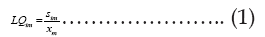
If the value of this ratio is greater than 1 then it indicates that region m is specialised in industry i. A value between zero and 1 indicates no specialisation. A value of the ration equal to 1 indicates that the share of industry i in region m is equal to the national average.
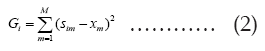
Concentration of industries: In contrast to this, the concept of industrial concentration within a country measures the overall concentration of an industry i across all M regions. In other words, it captures the degree to which the percentage distribution of industry i employment across M regions corresponds to the percentage distribution of employment across M regions. It is defined by equation (2) below,
Both these measures estimate the degree of industrial concentration without controlling for the within-industry distribution of plant. Ellison estimated the degree of concentration of industries across regions in excess of the plant-level concentration. They termed this index as index of industrial localisation or industrial agglomeration index.
Agglomeration of industries: While estimating the degree of agglomeration of an industry, constructed a discrete probability model following Bernoulli distribution to analyze the correlation between the location choices of two plants belonging to the same industry. The two plants within the same industry may locate near each other due to the presence of externalities or spillovers. In this paper, spillovers have been defined in terms of benefits from exchange of labour pool within the same industry. A plant may choose to locate in a region where it can gain maximum profit.
The profit function of a plant belonging to industry i located in region m is affected by two factors-
a) employment share of region m in aggregate employment and the
b) location of other plants within the same industry owing to the presence of spillovers.
Letthere be N number of plants in industry i  and, are the share of these plants in the total employment (or output) of the industry. The Herfindahl index of industry i as
  captures the plant size distribution within industry i.
The model assumes that the location choice of plant j to set up its operations is an independent identically distributed
random variable  each taking values from 1,2,..........,M with probabilities
  The re-write regional share of industry i as,
 where um is the Bernoulli random variable which takes a value 1 if a plant j locates in region m, i.e. vm= m and 0 otherwise.
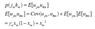
Ellison and Glaeser modelled the interaction between the location decision of two plants j and k within the same industry i owing to the presence of spillover. The interaction between the location decisions of two plants within the same industry in region m is defined as,
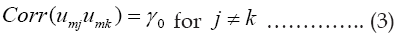
The γ captures the degree or the strength of spillover between two plants belonging to the same industry, located in the same region. The probability that plant j and k will locate in the same area m is given by,
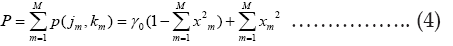
The probability P that plant j and k locates in any of the M locations is given by,
Spatially-weighted index of industrial agglomeration: Ellison index has been criticized, later for capturing the degree of concentration irrespective of its geographical position relative to other areas within the country i.e. spillover from adjacent regions was not considered in the estimation process. This can be elaborated with an example,
Suppose there are 12 plants within an industry located across 16 regions. Three hypothetical spatial distribution patterns of these 12 plants across 16 regions has been represented by the grids in (Fig. 1).
From the above distributional pattern and given the position of each region, it can be interpreted that the concentration is highest in Fig.1a based on the distance between any two pair of plants. The concentration is higher in Fig. 1b compared to Fig. 1c. However, the Maurel indices both are observed to have same value in all the above three cases as these indices captures concentration within a defined spatial unit, irrespective of its geographical position with the neighbouring regions.

Figure 1: Three hypothetical spatial distribution patterns of these 12 plants across 16 regions has been represented by the grids.
Maurel the index of industrial agglomeration has been modified to incorporate the spillover effect of the neigh bouring regions (Maurel, et al., 1999). The spillover effect of economic activity of adjacent regions has been captured
by weighing the regional share in equation (5) by using the spatial weights matrix, W. The modified Ellison
Glaeser Index of agglomeration can be re-written as, 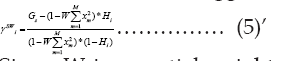
Since, W is a spatial-weight matrix so the equation (2)’ can be re-written in the vector form as,
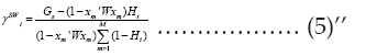
where, 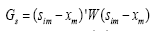 is the Spatially weighted Gini Index
of equation (1).
is the Spatially weighted Gini Index
of equation (1).
Features of Industrial Agglomeration in India
States with highly developed industrial base are also hub of some of the highly polluting industries: While analyzing the spatial development process of the organized manufacturing sector, it has been observed that there is an inequality in the distribution of the manufacturing output across states. In the year 2013-14, states like Tamil Nadu, Maharashtra, Uttar Pradesh, Gujarat and Haryana together accounts for 60% of the total manufacturing output produced in the economy. While analysing the nature of industrial development, it has been observed that industries (defined at the 4-digit level NIC2008) like manufacturing of sugar, tanning and dressing of leather, paper and pulp, pharmaceutical, basic iron and steel, basic chemicals show a high degree of specialisation (LQ>1; as defined by equation 1 in the previous section) in these states, baring Haryana. According to the definition of CPCB, these are the highly polluting industries and are defined under the Red Category (CPCB 2016).
As opposed to this, the nature of industrial development in Haryana, Karnataka and Chandigarh has been less polluting. Industries like manufacturing of parts and accessories of motor vehicles, fabricated metal products, electronic components, transport equipment’s, categorized under the Green category by CPCB, show a high degree of specialization in these states.
Total manufacturing industries of about 44% of the (defined at the four-4digit level of nic2008) are found to be highly agglomerated in the year 2013-14: The degree of agglomeration of Indian manufacturing sector has been estimated by using the EG Index as defined by equation (5) in the previous section. If the value of is below 0.02 but positive, then the industry is not very agglomerated. If the value of varies between 0.02 and 0.05 then the industry is moderately agglomerated and if value of is above 0.05 then the industry can be categorized as highly agglomerated. The negative value of indicates that the industry is dispersed.
Using this definition, it can be observed from Fig. 2 below, that 44% of the total four-digit industries included in the study are highly agglomerated, 30% are moderately agglomerated and 26% of the industries are either dispersed or have lower degree of agglomeration.

Figure 2: Distribution of the degree of industrial agglomeration in the year 2013-14
Some of the top agglomerated industries, identified at the 4-digit level of industrial classifications are listed in the Table 4 below. It can be observed that the agglomerated industries also have a high Gini Index (GUNW) which captures the geographic concentration of the industry. However, it is not true that the all agglomerated industries have high degree of plant-level concentration within an industry, captured by the Herfindahl Index (H) in the second column of the above table. For example, tanning and dressing of leather have a high degree of geographic concentration (GUNW) with a value of 0.22 but the within-industry plant structure (H) seems to be dispersed with a value of 0.004.
| Industry | EG | Technology Category | Pollution Category |
|---|---|---|---|
| Manufacture of pulp, paper and paperboard | 0.0004 | Low tech | Red |
| Manufacture of structural metal products | 0.0066 | Medium-low tech | Green |
| Manufacture of rubber tyres and tubes | 0.007 | Medium-low tech | Red |
| Manufacture of motor vehicles | 0.0076 | Medium-high tech | Green |
| Manufacture of optical instruments and equipment | 0.0084 | High-tech | Green |
| Manufacture of machinery for mining | 0.01 | Medium-high tech | Green |
| Manufacture of electric motors, generators | 0.0102 | Medium-high tech | White |
| Manufacture of batteries and accumulators | 0.0116 | Medium-high tech | Red |
| Manufacture of soft drinks | 0.0137 | Low tech | Orange |
| Manufacture of furniture | 0.0142 | Low tech | White |
| Manufacture of fertilizers and nitrogen compounds | 0.015 | Medium-high tech | Red |
| Manufacture of plastics products | 0.0229 | Medium-low tech | Green |
| Manufacture of electronic components | 0.0242 | High-tech | Green |
| Manufacture of communication equipment | 0.0253 | High-tech | Green |
| Manufacture of made-up textile article | 0.0315 | Low tech | Green |
Table 4. Nature of least and moderately agglomerated industries
This indicates that overall agglomeration; captured by EGUNW of tanning and dressing of leather industry is primarily driven by the geographic concentration and not by the underlying plant-structure. Some of the least agglomerated industries in the manufacturing sector in the year 2013-14 are manufacturing of dairy products, manufacturing of structural metal products, manufacturing of pulp and paper etc. It has been observed that manufacturing of machinery for metallurgy, computer and computer peripherals, man-made fibres are some of the dispersed industries (EGUNW <0) in the year 2013-14 in Table 5.
| Industry | EGUNW | Herfindahl | GiniUNW |
|---|---|---|---|
| Manufacture of bicycles and invalid carriages | 0.531 | 0.023 | 0.543 |
| Manufacture of tobacco products | 0.418 | 0.027 | 0.451 |
| Manufacture of knitted and crocheted apparel | 0.392 | 0.004 | 0.395 |
| Manufacture of other porcelain and ceramic products | 0.332 | 0.009 | 0.337 |
| Processing and preserving of meat | 0.248 | 0.032 | 0.264 |
| Manufacture of carpets and rugs | 0.24 | 0.012 | 0.252 |
| Manufacture of leather luggage, handbags etc. | 0.238 | 0.011 | 0.246 |
| Manufacture of jewellery and related articles | 0.231 | 0.033 | 0.238 |
| Manufacture of sports good | 0.224 | 0.045 | 0.265 |
| Tanning and dressing of leather | 0.216 | 0.004 | 0.222 |
| Manufacture of railway locomotives and rolling stock | 0.194 | 0.026 | 0.227 |
| Finishing of textiles | 0.182 | 0.003 | 0.183 |
| Manufacture of coke oven products | 0.181 | 0.028 | 0.196 |
| Manufacture of other chemical products n.e.c. | 0.176 | 0.005 | 0.177 |
| Manufacture of other transport equipment n.e.c | 0.149 | 0.119 | 0.202 |
Source: Author’s calculation based on ASI-factory level database
Note: UNW: Spatially unweighted index
Table 5. Top 15 Highly Agglomerated industries in the year 2013-14.
Most of the low-tech polluting industries show a high degree of industrial agglomeration: While analyzing the nature of industrial agglomeration, it has been observed that the average degree of agglomeration of polluting industries is greater than the average degree of agglomeration of non-polluting industries in Table 6. Below lists some of the highly agglomerated (EG>0.05) polluting and non-polluting industries in the Indian organised manufacturing sector in the year 2013-14. It is apparent from the table that most of the low-tech polluting industries are highly agglomerated (Ghani, et al., 2014). Table 6. Nature of highly agglomerated industries
| Industry | EGUNW | Technology Category | Pollution Category |
|---|---|---|---|
| Manufacture of tobacco products | 0.418 | Low tech | Red |
| Manufacture of knitted and crocheted apparel | 0.392 | Low tech | Green |
| Manufacture of other porcelain and ceramic products | 0.332 | Low tech | Red |
| Processing and preserving of meat | 0.248 | Low tech | Red |
| Manufacture of carpets and rugs | 0.24 | Low tech | Green |
| Manufacture of leather luggage, handbags | 0.238 | Low tech | Green |
| Tanning and dressing of leather | 0.216 | Low tech | Red |
| Finishing of textiles | 0.182 | Low tech | Red |
| Manufacture of coke oven products | 0.181 | Medium-low tech | Red |
| Manufacture of other chemical products n.e.c. | 0.176 | Medium-high tech | Red |
| Manufacture of other food products n.e.c. | 0.141 | Low tech | Red |
| Manufacture of office machinery and equipment | 0.131 | High tech | Green |
| Manufacture of other textiles n.e.c. | 0.128 | Low tech | Red |
| Manufacture of basic chemicals | 0.125 | Medium-high tech | Red |
| Manufacture of footwear | 0.117 | Low-tech | Green |
Source: Author’s calculation based on ASI-factory level database
Table 6. Nature of highly agglomerated industries
Neighbourhood effect’ affects the degree of industrial agglomeration: The degree of industrial agglomeration has been estimated by using the EG Index as represented by equation (5) as described in the previous section. However, the formulation of the index does not capture the degree of spatial concentration of an industry i.e. concentration relative to other adjacent regions within the country. Moreover, it has been calculated based on the employment data of each industry across states, where states are pre-defined by boundaries. The degree of industrial concentration calculated in this manner, may suffer from a downward bias as this cannot capture the effect of adjacent regions. The bias has been corrected by estimating the spatially weighted agglomeration index as indicated by equation (5)'' for all the 125 four digit industries included in our sample. The spatially weighted (EGSW) and spatially unweighted EG (EGUNW) are positively and highly correlated (the coefficient of correlation is 0.88 significant at 5% level of significance), as depicted by the scatter diagram in (Fig. 3A).

Figure 3A: Excess concentration in manufacturing of man-made fibers

Figure 3B: Excess concentration in manufacturing of machinery for metallurgy
The manufacturing of man-made fibres (NIC -2030) seems to be clustered in the northern, north-eastern and eastern region of India. The manufacturing of machinery for metallurgy (NIC-2823) appears to be clustered in the north-western region. It also appears to be clustered in a small pocket in the eastern region.
This analysis indicates that EG index cannot capture the degree of spatial agglomeration and may lead to misleading conclusion about the degree of industrial agglomeration. While analysing the impact of industrial agglomeration it is pertinent to modify the index by weighing it with the spatial matrix. In this study, all the analysis in the following papers has been conducted based on the EGSW.
Spatial Evolution of Industrial Agglomeration- 2000-01 vs. 2013-14
Evolution of manufacturing activity across states: During the period of analysis (2000-01 to 2013-14), the total output of the organised manufacturing sector has registered a growth of 0.151% accompanied by a moderate employment growth (0.039%) in the sector. While analysing the distribution of manufacturing activity across Indian states, it is true that the share of the already industrialised states like Gujarat, Maharashtra, Andhra Pradesh and Uttar Pradesh constitute the bulk of the total manufacturing output. However, during this period it is noteworthy to observe that some of the industrially laggard states like Jammu and Kashmir, Meghalaya, Uttarakhand, and Himachal Pradesh, have registered a high growth rate in terms of both the manufacturing output as well as employment. This is reflective of the fact that over time organised manufacturing activities has been spreading across states.
While analysing the nature of this spread, it has been observed that some of these states like Jammu and Kashmir and Meghalaya have experienced an increase in the share of polluting industries in their total manufacturing output. Fig. 4A and 4B below compares the degree of specialisation of polluting industries between 2000-01 and 2013-14 across Indian states. It appears that states like Maharashtra and Rajasthan were specialised in polluting industries in the year 2000-01 but over the period they show a declining trend in the degree of specialisation in polluting industries. States in the north-eastern and eastern region of India over both the period specialises in polluting industries. It seems like the industrial core regions (baring, Gujarat and West Bengal) have been shifting towards production of cleaner output at the expenses of the peripheral regions of the country, generally characterised by lax environmental regulations. However, it is not possible to comment anything on the possibility of pollution haven effect across Indian states from this analysis and it is beyond the scope of the present study but this could be a possible hypothesis for future scope of research.

Figure 4A: Location quotient of polluting industries in 2000-01

Figure 4B: Location quotient of polluting industries in 2013-14.
Evolution of manufacturing activity across industries: The average degree of industrial agglomeration in both the time 2000-01 and 2013-14 indicates that manufacturing industries in India are highly agglomerated; with EGUNWavg (2000-01) as 0.111 and EGUNWavg (2013-14) being 0.071 respectively. However, over time, the degree of concentration has declined, indicating the dispersion of industries across space. While distinguishing between polluting and non-polluting industries, it has been observed that during 2000-01 to 2013-14, the dispersion of polluting industries has been higher as opposed to the non-polluting industries. In the below lists some of the polluting industries for which the degree of agglomeration has declined in the year 2013-14 compared to its degree of agglomeration in the year 2000-01 in Table 7.
| Industry | EGUNW (2013-14) | EGUNW (2000-01) | ∆EGUNW | ∆EGSW |
|---|---|---|---|---|
| Manufacture of coke and oven products | 0.181 | 0.472 | -0.29 | -0.285 |
| Processing and preserving of meat | 0.248 | 0.474 | -0.227 | -0.421 |
| Forging, pressing, stamping | 0.047 | 0.222 | -0.175 | -0.203 |
| Manufacture of plastics and synthetic rubber in primary forms | 0.083 | 0.229 | -0.146 | -0.172 |
| Manufacture of other chemical products n.e.c | 0.176 | 0.304 | -0.128 | -0.1 |
| Manufacture of basic Chemicals | 0.125 | 0.198 | -0.073 | -0.055 |
Source: Author’s calculation based on ASI factory-level data
Note: ∆EGSW: [EGSW (2000-01) - EGSW (2013-14)]
Table 7. Change in the degree of industrial agglomeration of polluting industries
It is true that polluting industries show a declining trend in their degree of agglomeration over time, but these are some of the highly agglomerated industries (EG>0.05) in the year 2013-14, also reported in Table 8. The decline in the EG index over time especially in case of polluting industries indicates the presence of diseconomies or negative spillover among the plants−initiating dispersion forces. The last column of the table indicates that over time spatial agglomeration (EGSW) has also declined for these industries.
| Ratio a:EGUNW/EGSW | Number of Observations:125 | ||
|---|---|---|---|
| a | Ratio | Linearized Std. Err. | [95% Confidence Interval] |
| 0.50767 | 0.0329764 | 0.4424049 0.5729439 | |
Table 8: Ratio estimation of EGUNW/EGSW.
The analysis in this paper confirms the fact that there are agglomeration economies (or diseconomies) in terms of sharing of sharing of labour across plants among the organised manufacturing industries. The impact of these economies and diseconomies has been empirically examined further in the following two papers of the thesis (Fig. 5).

Figure 5: Scatter plot between EGUNW and EGSW
The distribution of the organised manufacturing sector has been uneven across Indian states indicating a core-periphery dichotomy pattern of industrial development within the country. States like Tamil Nadu, Maharashtra, Uttar Pradesh, Gujarat and Haryana together constitutes the bulk of the total manufacturing output produced in the organised sector. During the period of the analysis i.e. between 2000-01 and 2013-14, the bulk of the output has remained confined within the already industrialised states. However, it is noteworthy to observe that during this some of the industrially laggard states like Uttarakhand, Jammu and Kashmir, Himachal Pradesh have registered a high growth in terms of both manufacturing output as well as employment. This indicates that manufacturing activities has been spreading over time across states. While analysing the nature of industries it has been observed that these laggard states over time has actually gained in terms of the share of polluting industries in their total manufacturing output. In contrast to this, some of the industrial core regions like Maharashtra and Rajasthan have registered a declined in the share of polluting industries in their total manufacturing output. Is it true that over time the industrially advanced states characterised by stringent environmental regulations are becoming cleaner at the expense of the environmental degradation of the peripheral states in India? indicating a pollution haven effect across Indian states. However, this needs further analysis and can be a potential for future scope of research.
The paper uses the annual survey of industries factory-level data to estimate the degree of industrial agglomeration in the Indian manufacturing sector based on the plant-level employment data. It has been observed that irrespective of the nature of industries there exists a high degree of agglomeration economies among manufacturing industries. The underlying economies arsing from the sharing of labour across manufacturing plants indicate that clustering of industries may accentuate the employment growth of the sector. However, the evidence of high agglomeration among the low-tech polluting industries raises concern about the environmental impacts associated with the clustering process. This entails cost-benefit analysis during the formulation of the industrial clustering policies. Moreover, it seems imperative to have information on industry-specific degree of concentration within a state as well as in the adjacent states (as indicated by the ‘neighbourhood effect’ in the analysis). This in turn will facilitate formulation of industry and region-specific policies to mitigate the environmental problems associated with the industrial clustering.
Copyright © 2026 Research and Reviews, All Rights Reserved