
ISSN (0970-2083)
ISSN (0970-2083)
VaibhaV Singh Rajput1*, Ravi Kumar Jatoth2, Nagu Bhookya3 and Bhasker Boda4
1Department of Metallurgy and Materials Engineering, National Institute of Technology, Andhra Pradesh, India
2Assistant Professor, Department of Electronics and Communication, National Institute of Technology, Warangal, India
3Assistant Professor, Department of Electrical Engineering, National Institute of Technology, Warangal, India
4Assistant Professor, Department of Electronics and Communication Engineering, K.G Reddy College of Engineering, Hyderabad, India
Received Date: 07 August, 2017 Accepted Date: 20 September, 2017
Visit for more related articles at Journal of Industrial Pollution Control
In this paper proportional, integral, derivative (PID) controller is used to control the pitch angle of the aircraft when the elevation angle is changed or modified. The pitch angle is dependent on elevation angle; a change in one corresponds to a change in the other. The PID controller helps in restricted change of pitch rate in response to the elevation angle. The PID controller is dependent on different parameters like Kp, Ki, Kd which change the pitch rate as they change. Various methodologies are used for changing those parameters for getting a perfect time response pitch angle, as desired or wished by a concerned person. While reckoning the values of those parameters, trial and guessing may prove to be futile in order to provide comfort to passengers. So, using some meta heuristic techniques can be useful in handling these errors. Hybrid GA-PSO is one such powerful algorithm which can improve transient and steady state response and can give us more reliable results for PID gain scheduling problem.
Pitch rate, Elevation angle, PID controller, GA, PSO, Phugoid
These days aircraft, jets, missiles mainly rely on automatic modes for its convenienceprovided to the passengers and to the pilot himself. However, theseautomaticcontrol systems need to be accurate and fast enough to respond. The control of aircraft pitch is dependent on deflection of elevator hinged at the tail of aircraft. The deflection causes the air to get redirected. This causes a force and as a result aircraft revolves about the pitch axis. The elevator is displaced by a control stick. The elevator deflects in proportion to the stick (deg) and resulting rotation about the pitch axis is called pitch rate measured in degree of rotation per second (deg/s) (Cadwell, 2010). The dynamics of aircraft control system comprises of longitudinal and lateral directions.
The pitch control is a longitudinal control. (Vishal and Jyoti, 2014) Hence, our focus will be only in the longitudinal model and longitudinal equations of motion. In past many researchers have done work in order to control the pitch, yaw and roll angle of the aircraft (Amit and Sharma, 2009; Vishal and Jyoti, 2014; Saad, et al., 2012; Wahid and Rahmat, 2010).
This paperfocuses on PID controller tuning with GA,PSO and hybrid GA-PSO to control the pitch rate of the aircraft. Using PSO algorithm can be a smart choice as it is fast and converges very quickly. (Karaboga and Okdem, 2004) However, on the other hand, there is high possibility of PSO to get stuck on the local values rather than searching for a global value. This problem is eliminated in GA as it doesn’t converges on a local value and hunt for global values.
The very problem GA offers is, slow convergence rate for computationally expensive functions. (Eberhart and Shi, 2000; Musrrat, et al., 2009) In order to overcome these complications hybrid of PSO and GA proved to be a better alternative. The speed of PSO merged with the global hunting characteristics of GA can bring out the best solution within a limited time and iterations. Hybrid GA-PSO when tuned for PID parameters for pitch rate detection gave much better results than GA and PSO alone. The simulation is done in MATLAB and SIMULINK for the analysis of PID parameters. The rise time, settling time, steady state error, maximum overshoot are calculated for these algorithms and are compared.
The feedback eliminates error but gives poor transient and steady state response (Figure. 1). This is improved by PID controller. The comfort for the passengers includes:

Figure 1: PID block diagram in feedback loop.
1. Overshoot less than 10%.
2. Rise time less than 2 sec.
3. Settling time less than 10 sec.
4. Steady state error less than 2%.
e (t) = r (t)-y (t) ……. .(i)
 (ii)
(ii)
Where, r (t) is the require value, y (t) is the output value and e (t) is the error, u (t) is the new value PID converts error.
Then error (e (t)) of the plant isoptimized using PID controller which is then optimized using metaheuristics techniques as mentioned earlier. These requirements for plant are not fulfilled without using PID controller. The PID controller is placed in a control loop feedback mechanism used to evaluate error continuously between desired value and measured variable. The PID controller tries to reduce error by using its three parameters Kp, Ki, Kd, Kp term accounts for the present value of error. Ki term accounts for the past values of error. Kd term accounts for the future values of error.
Setting values for these parameters is called tuning of the PID parameters. Trial and error method can give results but can become cumbersome and does not guarantee perfect values. Hence, tuning is required to set the PID parameters.
The equations of motion of aircraft can be divided into lateral and longitudinalequations. As stated earlier our major concern will be mainly on longitudinal direction and its equation (Torabi, et al., 2013; USAF, 1988).
Descriptionof pitch conduct
The pitch control of aircraft can be thought as a combination of two second order transfer equation, describing short and long period stability characteristics called modes (Cadwell, 2010). The combination of two, results in 4th order transfer function.
The long period mode called the phugoid is a nondivergent oscillation of aircraft (time period greater than 10 seconds) about the pitch axis (Figure. 2). This term is only present when the aircraft is positively stable and simplifies into divergence if it is negatively stable (USAF, 1988; Cadwell, 2010). This divergence can be ignored in comparison to the short period mode as its effect is greater than long period mode. So, we will negotiate long period oscillation for these reasons. Eliminating long period oscillation restricts our work and equation to second order transfer function (Liu and Lampinen, 2002).

Figure 2: Phugoid mode.
Equations of motion
The equations of motion of aircraft are very complex and complicated to understand. Hence, in order to apply these equations some modifications could be beneficial. The developments of equations are shown below (Figure. 3):

Figure 3: Viewing axis of aircraft x, y, z from ground frame with X, Y, Z axis of ground.
Translational motion equation
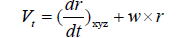
From Newton’s second law, applying from ground frame (Figure. 4):

Figure 4: Pitch axis(y axis), Roll axis(x axis), Yaw axis(z axis). Where w= Net Angular velocity of Aircraft; Vt =Total velocity (True Velocity) of Aircraft; m=mass of the aircraft.
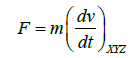 (1)
(1)
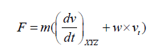 (2)
(2)
Taking components of w and in roll, pitch,yaw axis:
Hence,
 (3)
(3)
where, p, q, r are angular velocities in x, y, z direction
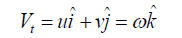 (4)
(4)
Where, u, v, ω are velocities in x, y, z direction
By using equations, (1), (2), (3), (4)
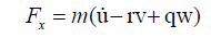 (5)
(5)
 (6)
(6)
 (7)
(7)
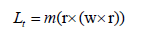
Rotational motion equation
 (8)
(8)
where, Lt=Total angular momentum of aircraft r = Position vector from the center of gravity of aircraft.
 (9)
(9)
 (10)
(10)
As m is variable on the whole aircraft, integrating angular momentum for a dm mass (Figure. 4), over the whole aircraft will bring out the net angular momentum,
 (11)
(11)
Where, σ is the mass density of aircraft, which is same everywhere
V is the Volume of aircraft On solving equation (11)
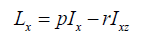
 (12)
(12)
 (13)
(13)
 (14)
(14)
Where, Ix, Iy, Iz are the moment of inertia about their respective axis
Using Newton’s rotational equation,
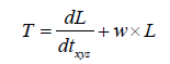 (15)
(15)
As most aircraft have plane of symmetry about x-z plane, so
Ixy= 0, Izy=0;
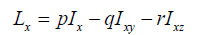
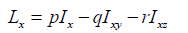
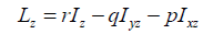
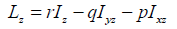
Then equations (12),(13),(14) changes to
 (16)
(16)
 (17)
(17)
 (18)
(18)
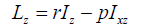
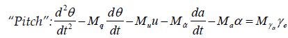
On putting these values to eq. (15) results into
Where, L, M, N are Torques/Moments about roll, pitch, yaw axis.
Relation between angles and angular velocity
Ψ = angle of yaw
Θ = angle of pitch
Φ = angle of roll
ϒe = angle of elevation
α = angle of attack
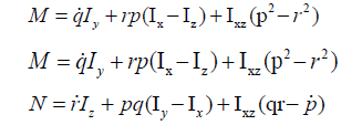
Calculating angles (also called Euler’s angles) relation with respective angular velocity can be done by taking one of the angles as zero for each axis and solving each axis mechanics. Then adding all relations result in equations:
 (19)
(19)
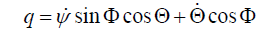 (20)
(20)
 (21)
(21)
The aircraft is mostly dependent on its aerodynamic terms for its motion. However, the above equations are that results from summing forces and moments, which are non-linear, and exact solutions are impossible. In order to linearize them a linearized model is suggested which is based on small disturbances and small perturbation theory. This model gives a boost to engineering problems because aerodynamic effects are linear functions of variables of interest.
To cap it all, the small disturbance theory is applied in three steps,
1. Write equilibrium conditions.
2. Assuming it has small perturbations.
3. Use first order Taylor series expansion to determine small perturbations effect.
When operating under small perturbation, longitudinal motion can be expressed in terms of variables shown:
• Longitudinal Motion
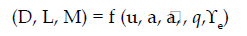
Where, D, L, M are Lift, Drag and moment in longitudinal direction
Applying small disturbance theory on above equations by substituting:
u=uo+δu; v=vo+δv; ω=ωo+ δω;
P=po+δp; q=qo+δq; r=ro+ δr
γ= γo+δγ;
For convenience we have assumed symmetric flight conditions and no propulsive forces are acting.
This implies vo=ωo=po=qo=ro= γo=0;
Using thrust, gravity and gyroscopic effect on D,L,M and applying Taylor series on those and equating them with the above equations of force and moment results in longitudinal direction equations.
Longitudinal motion equation
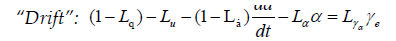 (22)
(22)
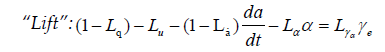 (23)
(23)
 (24)
(24)
As we stated earlier, longitudinal motion is what we care for, now writing equations for longitudinal direction for short period time (mode) in space state model:

y = Cx + Du
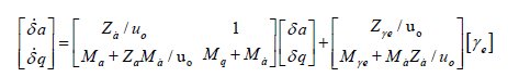 (25)
(25)
 (26)
(26)
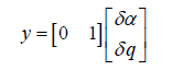
where y is the output matrix
Now, heading towards our transfer function:
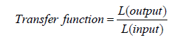
Now, using Cramer’s rule, transfer function can be evaluated for pitch rate and elevation angle using (25), (26):
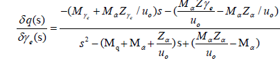 (27)
(27)
Also,  (28)
(28)
δq=sδΘ (29)
Hence, transfer function for pitch angle and elevation angle is,
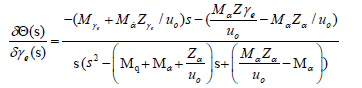
Now simplifying the transfer function by substituting values of variables from Table 1, (values taken from commercial Boeing aircraft).
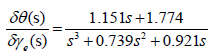 (30)
(30)
Optimization technique requires complicated techniques in order to accomplish the task. One of the technique in order to accomplish optimization is genetic algorithm (GA). GA is expectionally good at giving optimized results. GA involves a very famous concept of humanity “Survival of the Fitttest”. GA uses this concept to find the global values of the functions using chromosomes as its population, whose fitness is to be examined for survival. It involves three major process selection, mutation and crossover. The algorithm involves the following steps:
(i) Generation of Chromosomes
Randomly generated chromosomes in binary or real form are taken as the functions positions. These positions are used for testing the values and are further evaluated accordingly.
(ii) Mutation and Crossover
The generated chromosomes are then mutated and crossovered with each other to include every possibility to find the fittest chromosomes. All the generated, mutated and crossovered chromosomes are then taken for final selection to get the most fit population.
(iii) Selection
The pool of chromosomes generated using randomness, mutation and crossover are then selected to get the best generation of chromosomes. The best fit chromosomes give the best cost i.e. the global best.
The criticism GA and DE suffered of being slow was overcome by PSO as it has a very fast convergence rate. However, with this overwhelming speed one problem couldn’t be overcome i.e. sticking to a local value. This method is based on swarm behavior in nature. All swarms spread in all direction in order to find food (in this case global value). One that finds food calls other swarms to come to that place. This is exactly how particle algorithm works. These methods are also called nature inspired algorithms, as they are inspired from nature and its behavior.
The positions and velocities are generated randomly. Then they are updated according to the equations:
vt+1=yt*w*rand+c1*rand*(pbest–xt)+c2*rand*(gbest– xt) (31)
xt+1= xt+vt (30)
Where, w is inertial mass ÃÂÃâ[0,1], pbest is the personal best position, gbest is the global best position for the swarm, rand is any random number.
c1, c2 are self-confidence and swarm-confidence respectively.
The pseudo code for PSO is given below:
start:
Initialization position, velocity, personal best, global best
while {
Check the cost of function
Update personal and global best, if cost < previous cost
Update positions
Update velocities
Choose the best cost swarm positions}
End
In aircraft dynamic plant Kp, Ki, Kd are taken as 3-D positions. In (Figure. 5), PSO is checking the cost of function by passing positions (Kp, Ki, Kd) to plant and checking the best solution by optimizing error.

Figure 5: Implementation of GA-PSO in aircraft dynamic plant.
This algorithm can be applied to various engineering fields like control systems, intelligent systems, path planning, tuning of LQR and PID controllers.
After analyzing GA and PSO alone, one fact that cannot be put aside is that both have some or the other problem. This made GA, PSO algorithms to go futile in various fields. However, when combined effects of both are used, it gave much better results in terms of time and values.
First the best population of GA is sorted on the basis of its fitness. Then the best value for each vector is matched, with its fitness. Then those vectorpositions with their best values are passed to PSO. PSO searches for global values on the positions of those vectors and not randomly as it used to do earlier. The flow chart for hybrid GA-PSO and how it is applied to the aircraft dynamics plant is given in (Figure. 5).
PID parameters are calculated using the above methodologies. (Figure. 6) The error which is to be optimized is ISTE (Integral square time error), given by:

Figure 6: Simulink model.
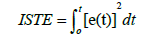 (31)
(31)
The error and tuning of PID parameters is done by using the above algorithms. The error form ISTE is optimized for getting the rise time, settling time, steady state error and maximum overshoot. The pitch angle (for open loop) graph on applying step response is shown (Figure. 7):

Figure 7: Open loop response for pitch angle vs. time.
The above graph doesn’t meet with required design (given in problem formulation) so, using PID may alter the results and can bring closer to desired model (Figure. 8).

Figure 8: Closed loop response for pitch angle vs. time.
The (Figure. 9) shows that both the poles are on the left side of imaginary axis. Hence, the function /plant is stable.

Figure 10: Comparison of GA, PSO, GA-PSO.
The PID parameters were obtained using PSO, GA, hybrid GA-PSO algorithms. Best results were noted for hybrid GA-PSO. The input (required value) response taken was 0.2 radians (11.2°). The comparison of all the algorithms is given in Table 2 and (Figures. 6 and 10). PSO and GA alone didn’t provide good settling time for pitch control of aircraft. Passengers comfort needs reduction in rise time, settling time, steady state error and maximum overshoot of closed loop response. These design requirements were met using nature inspired algorithms rather than arbitrary choosing values of Kp, Ki, Kd, which is clearly seen in Table 2:
Aircraft pitch control plant has been designed and analyzed carefully. Hybrid GA-PSO based controller has given the best results of all algorithms. The desired input given is 0.2 rad (11°deg). The rise time is 0.18 s the settling time is 0.32 s, maximum overshoot is 1.794%, and steady state error is 2.34 × 10⁻⁷. The results in Table 2, justifies thathybrid GA-PSO is the best method by far in order to optimize the pitch control of aircraft..
Copyright © 2026 Research and Reviews, All Rights Reserved