
ISSN (0970-2083)
ISSN (0970-2083)
Essombo C1, Jean Calvin Seutche1,2*, Bickelle Ambassa Georges1,2, Achille Clovice Goune1, Jean Luc Nsouandele3, Germain Hubert Ben-Bolie4, Atangana Jacques1,2
1Electrical and Electronic System Laboratory, University of Yaoundé I-Cameroon, Yaoundé, Cameroon
2Department of Physics, University of Yaoundé I-Cameroon, Yaoundé, Cameroon
3National Advanced School of Engineering Maroua, University of Maroua–Cameroon, Maroua, Cameroon
4Laboratory of Atomic, University of Yaounde, Yaounde, Cameroon
Received: 26-Oct-2022, Manuscript No. ICP-22-78209; Editor assigned: 01-Nov-2022, PreQC No. ICP-22-78209 (PQ); Reviewed: 15-Nov-2022, QC No. ICP-22-78209; Revised: 23-Nov-2022, Manuscript No. ICP-22-78209 (A); Published: 30-Nov-2022, DOI: 10.4172/0970-2083.003
Visit for more related articles at Journal of Industrial Pollution Control
The concerns about the origin of environmental pollution, derived from anthropogenic activities at industrial sites, are a major issue worldwide. Therefore; it will be important to look at the origin of these different entities that create this disorder. This article deals with the simulation of the identification of polluting sources from the Oyom-abang thermal power plant (CTO) using the Gaussian method. The aim is to highlight the different species from this plant that contribute effectively to the destruction of the atmosphere. These polluting species, which are easily dispersed in the atmosphere, are identified from their concentrations measured in kg m-3 . The measurement of the concentration of pollutants emanating from the point sources of pollution with the help of sensors was done in two and three dimensions (2D and 3D). The identified sources were represented in three dimensions (3D). The Gaussian model was used as a puff model to obtain the shape of the solution in a local scale. Fortran software was used to compile the numerical scheme of the advection-diffusion equation using the finite difference method centered in space and time. Finally, the MATLAB2016a software allowed us to obtain the results and position the sensors for efficient identification of the concentration from the source to be identified. For a more efficient identification of air pollution point sources, the optimal positioning of the sensors must also be determined. The Gaussian method is a reliable method for the study of pollution source identification at a local scale. Its simulation domain extends from 1 to 10 km and its applications are summarized on local impact and industrial risks.
Air pollution, Gaussian model, Thermal power plant, Identification
In Cameroon, 13.6% (Eneo, 2017; 2018) of electricity production is provided by thermal power plants. During this production, several mechanisms are set up. The gases and pollutants released into the atmosphere, allow us to have a generalized knowledge of calm weather and a high frequency of clear skies (Cervone and Franzese 2011; Michelot et al., 2015); which will then favor the establishment of temperature inversion and confer a ventilation essentially provided by the thermal breeze fire. However, other circumstances that can also lead to uncontrolled releases of pollutants into the atmosphere are varied: these include accidental situations, for example leaks or explosions on an industrial site or in a land environment (Tchindjang et al., 2001; Bocquet et al., 2011). Faced with such situations, the objectives of the authorities are multiple: to anticipate the impacted areas in the short term, in particular to evacuate the populations concerned; to locate the source in order to be able to intervene directly on it; and finally, to identify and characterize the source of pollution. This problem encountered by the local population has led some researchers to attempt to monitor the concentration of air pollution more precisely in order to inform the people concerned (James et al., 2011; Chaiwino et al., 2021).
The concerns about air pollution are increasing worldwide (Azad and Kitada, 1998; Cahier et al., 2005; Debananda et al., 2015). It is well known that industries such as thermal power plants, power stations, automotive industries, etc., are the most major sources of pollution especially in the atmosphere (Arnesen and Krogstad, 1998; Stevens et al., 1998). These pollutants and gases released into the atmosphere vary considerably in their composition. Pollution is currently a major concern for all countries around the world, as they are small enough to penetrate deep into the lungs and easily cause disasters (WHO, 2013). However, if we are to be effective in our fight against pollution, we must first eradicate the roots of the problem rather than just treating the symptoms (Chaiwino et al., 2021). This means being able to identify the sources of air pollution and their corresponding characteristics. This data can be used by local authorities to issue a first warning to factories while allowing a thorough investigation of the causes and sources of the detected real-time pollution. Therefore, many researchers are interested in this topic (Chaiwino et al., 2021; James et al., 2011) and have started to improve some algorithms or models capable of efficiently specifying the exact positions of pollution sources. Our case study is the OYOM- ABANG thermal power plant located in the city of Yaounde-Cameroon, more precisely in the Centre region, department of Mfoundi and district of Yaounde VII (Fig. 1). The following study is therefore part of a doctoral research and is identified as a first approach for an inverse modelling work. To achieve these objectives, the Gaussian model will be used, as it is a non-parametric puff model that is part of a local scale study and has very simplifying and efficient assumptions. More recently, in order to achieve effective pollution management methods more precisely in the search for pollution sources identification, and satisfactory emergency responses; many results have been obtained concerning the improvement of the accuracy on information estimates of air pollutant emission sources. (Mallet and Sportisse, 2004) studied the 3-D chemistry-transport model Polair for identifying pollution sources: Strategic numerical problem validation and automatic differentiation by describing Polair as a three-dimensional transport chemistry model that is an efficient and robust solver for simulating emissions reconstruction on 8th March 2004 (Li et al., 2009) These techniques allow for online error estimation (Krysta et al., 2008), have worked on the Hansen L-curve technique in 1992 to estimate the r/m ratio for two parameters in the context of the Chernobyl inverse. In the same line (Bocquet et al., 2010) showed that even with a number of source parameters three times smaller than the number of observations, the poor observability of some variable sources still leads to an ill-conditioned problem with a very high sensitivity of the results to hyperparameters, such that a hyperparameter estimation technique is required. (Victor et al., 2011) have worked on error estimation in inverse modelling of accidental air pollutant releases: application in the reconstruction of source terms of caesium-137 and iodine-131 from the Fukushima Daiichi power plant in 2014 using the POLAIR model to identify radioactive sources. More recently (Cui et al., 2019; Li Hui et al., 2019; Chaiwino et al., 2021) have worked on Identification of air pollution source locations with models (Gaussian dispersion model and PSO model). Basic meteorological parameters such as wind speed, wind direction, temperature and precipitation cause the horizontal transport and dispersion of air pollutants (Ziomas et al., 1995; Li Hong et al., 2009; Moudi et al., 2011). In this research, the objective is to conduct a point source identification study in the oyom-abang thermal power plant based on the Gaussian bouffer model. We then apply the finite difference numerical method to solve the PDEs. In addition, the positioning of the sensors was also designed to increase the efficiency of the search. A brief systematic description of the Gaussian model is then given. The results of this study are discussed in the last section.

Figure 1: OYOM-ABANG in the city of Yaoundé-Cameroon. Note: ( ) Village; (
 ) Batiment; (
 ) Riviere; (
 ) Lac; (
 ) Vegetation; (
 ) Cameroon-de-Yaoundé.
Description of the Study Area
The OYAM ABANG district is located in the Centre region of Cameroon, so the space occupying the thermal power plant called OYO is an industrial site with an area of 1.38296 hectares. Its geographical coordinates are (Latitude: 03.52 to 51.7 on Longitude: E 011°28’00.6’’; producing electricity from heavy fuel oil and light fuel oil injected in the engines of the brand CATERPILAR3516B WARTSILA VASA 18V32LN. The company involved in this production is Eneo (Energy of Cameroon) (Seutche et al., 2015; Eneo, 2017; Eneo, 2018; Seutche et al., 2019). For this geographical environment, (Seutche et al., 2015) indicate, thanks to fixed and itinerant measurements of meteorological parameters, that the OYAM-ABANG basin experiences two local meteorological phenomena each day of the study period in the absence of a marked synoptic wind that is the rule in this region:
• The phenomenon of thermal breezes.
• The presence of a temperature inversion.
In addition, the flow of cold air along the slopes accentuates the inversion phenomenon and allows the installation of a thin, calm or weakly ventilated lake of cold air. The topographic configuration offers few escape routes for the cold air. It therefore accumulates at the bottom of the basin with the pollutants emitted (Fig.2).

Figure 2: National map of thermal power plants in Cameroon. Note: ( ) 225; (
 ) 110; (
 ) 90; (
 ) Lignes Distribution; (
 ) centrales thermiques interconnectees sub HFO; (
 ) centrales thermiques interconnectees sub LFO; (
 ) centrales thermiques interconnectees Nord; (
 ) centrales thermiques isolees Sub; (
 ) centrales thermiques isolees Nord; (
 ) centrales hydroelectriques; (
 ) Barrages reserviors; (
 ) centrales isolees hybride; (
 ) Producteurs independants
Equation Governing the Atmospheric Dispersion of Pollutants
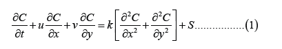
Atmospheric dispersion characterizes the future, in time and space, of a pollutant cloud from a source released into the atmosphere. Atmospheric dispersion modelling is the mathematical description of the advection-diffusion process. This process reproduces the behavior of the pollutant concentrations in the study area. The general advection-diffusion equation is:
In this work, we are interested in the behavior of point sources. For m points sources, the source term is given by:
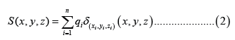
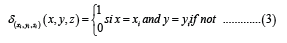
Where qi is the emission rate for i sources and the function δ(xi,yi,zi) (x,y,z) is defined:
The diffusion coefficients kx and ky represent the ability of the pollutant to pass through the median. Thus, these coefficients depend on the space variables, which means the area of the domain. In this study, we assumed that the pollutant is emitted in a homogeneous area, which means that these coefficients are constant and given by kx=13,8 and ky=10,2.
Numerical Methods
The choice of numerical simulation method depends on the problem studied, when it comes to numerical solution spaces, numerical methods are used for the evaluation of the gradient at each iteration, this is the case of the finite difference method. This simulation method exists in different forms and is presented here by the Fortran 97 software. The numerical solution of the equation aims to approximate the value of the concentration at each point (xi,yj,zk,tn) of the study domain and at each time tn+1 where tn= nΔt n =1, 2........... R The approximate value of this concentration is noted C (xi,yj,tn)=Cnij. The study area consists of a spatial grid x Δ , y Δ and z Δ where xi = iΔx, yj= jΔy and zk = kΔz i =1, 2...........N , j =1,2...........M , k =1, 2...........O
Characterization of the Problem
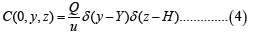
Initial conditions: The concentration is maximum at the stack exit for x = 0 . Thus, we have equation (4)
Problem area: We have as domainx∈[0;L] , y∈[0;L] , and z∈[0;L]
Boundary conditions: The concentration decreases as we move away from the source, therefore equation (4) becomes:
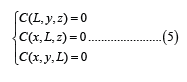
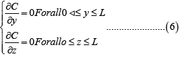
To eliminate the reflection phenomenon in y and z in equation (1), we then have the conditions for the flux:
Discretization of the Problem: Finite Difference Method
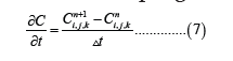
For this, we will use the classical numerical method known as the finite difference method. This method uses the regular calculation grid which has the advantages of ease of implementation and speed of calculation. To solve numerically this equation (1) we use the progressive method in time and space. For the unsteady term, we use the progressive differences:
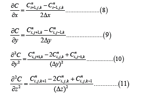
For the advection and molecular diffusion terms, center differences are used:
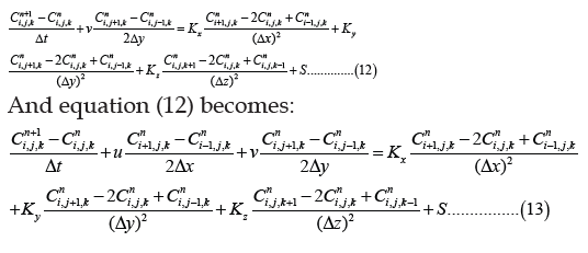
Equation (1) becomes:
And equation (12) becomes:
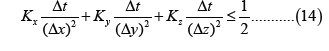
Stability condition:
Numerical models used: The dispersion model considered is a simple Gaussian plume model. This model has the advantage of low computational cost, the counterpart being a lower accuracy especially near obstacles, which are not taken into account. The Gaussian model is a representation of the concentration of pollutants in the air, the plume is emitted by a point source and is considered as a Gaussian distribution of the concentration. The Gaussian model is only valid for the following simplifying assumptions:
• A continuous point emission (active for a sufficiently long time to have a stable plume between the source and the furthest observed point), with a constant flow rate Q;
• Uniform wind fields (in speed and direction) in time and space;
• Atmospheric turbulence is constant in space and time;
• No obstacles, no relief.
The analytical solution being known and given by Fig. 3.

Figure 3: Analytical solution for identifying pollutant sources using the Gaussian method.
This figure represents an analytical solution for the identification of polluting sources on a horizontal plane with a mean wind speed of 3m.s-1 and a flow rate of 0, 231 kg.s-1. The improved structure of the algorithm for the Gaussian model is shown in Fig. 4 below.

Figure 4: Analytical solution for identifying pollutant sources using the Gaussian method.
The Main Inputs to the Model
The Gaussian model supports different modules and configuration options that allow the effects influencing source identification. A number of assumptions can thus be made for each model. In this work, tests have been carried out in order to adjust the modelling parameters to the local context. Some of these are outlined below.
Meteorological data: The meteorological preprocessor integrated in the Gaussian model calculates the atmospheric boundary layer (AL) parameters from different data sets, e.g., wind speed and direction, date, time, cloud cover, heat flux density and AL height, etc. The weather data used can be raw, hourly or from statistical analysis. An hourly sequential weather file (for the first six days of January, April and July 2021) was created from data measured by the Ekounou meteorological station (in the Centre region of Cameroon) and monitored by the Ministry of Transport. The parameters reported are: temperature, wind speed, direction and cloud cover (Fig.5).

Figure 5: Flow chart of a Gaussian model algorithm.
Show the daily temperatures and velocities for the first six days of January, April and July 2021. We select the first six days of each month because the daily variation in these data is not very large and these months were chosen to cover all seasons of the year in Cameroon. The highest temperatures are between 10 am and 3 pm and the lowest between 4 pm and 9 am; while the strongest winds are between 12 to 19 km/h and calm the rest of the time (Fig. 6-11).

Figure 6: Daily temperature for the month of January 2021. Note: ( ) 1 Jan; (
 ) 2 Jan; (
 ) 3 Jan; (
 ) 4 Jan; (
 ) 5 Jan; (
 ) 6 Jan.

Figure 7: Daily wind speed for the month of January 2021. Note: ( ) 1 Jan; () 2 Jan; () 3 Jan; () 4 Jan; () 5 Jan; () 6 Jan.

Figure 8: Daily temperature for the month of April 2021. Note: () 1 Jan; () 2 Jan; () 3 Jan; () 4 Jan; () 5 Jan; () 6 Jan.

Figure 9: Daily wind speed for the month of April 2021. Note: () 1 Jan; () 2 Jan; () 3 Jan; () 4 Jan; () 5 Jan; () 6 Jan.

Figure 10: Daily temperature for the month of July 2021. Note: () 1 Jan; () 2 Jan; () 3 Jan; () 4 Jan; () 5 Jan; () 6 Jan.

Figure 11: Daily wind speed for the month of July 2021. Note: () 1 Jan; () 2 Jan; () 3 Jan; () 4 Jan; () 5 Jan; () 6 Jan.
Each month, the daily average temperature as in (Moudi et al., 2011) varies between 19°C and 31.2°C, the cloud cover is 80% on average, the wind speed varies between 2 and 19 km/h in the west according to the wind rose in Fig. 7. The wind rose is related to a circle which can be divided into 4, 8, 16 or 32 parts. Like the trigonometric circle, the main directions are: North is 0 or 360°, east is 90°, and south is 180° and West 270°.
Identification de la Source Pollenate Dans le Domaine Bidimensionnel Dan’s la TPO
The identification of the location of point sources of air pollution is detected from the different sensors. To identify the emission source, the number of sensors and their positions are set for the same types of results, based on their coordinates described by (Winiarek et al., 2014; Chaiwino et al., 2021).
The positioning of the sensors is identified from the area where the concentration estimate is minimal or almost zero (Chaiwino et al., 2021), in order to observe the propagation of particles from the source in the impacted area. The identified particles are: firstly, greenhouse gases (carbon dioxide (CO2), nitrous oxide (N2O) and methane (CH4)); secondly identified pollutants such as SOx, Nox; thirdly Meta Particles (PM1, 2, 5 and PM10); fourthly PAHs and finally VOCs. The three sensors chosen for the visualization of the pollutants are such that: the middle sensor is the main one followed by the left and thus the bottom one which will be able to effectively identify the pollutant from the first visible iso concentration or the identified concentration would be of the order 10-5 kg.m-3.
The results of the sensor location for point source identification in the Oyom-abang Thermal Power Plant (TPO) are presented in Figs.12-14.

Figure 12: The result of the determination of the location of the air pollution point source at a distance of 400 m from the pollutant or gas dispersion. Note: (  ) Atmosphere; (
 ) Sensors; (
 ) Exact location

Figure 13: The result of the determination of the location of the air pollution point source at a distance of 380 m from the dispersion of the pollutant or gas. Note: () Atmosphere; () Sensors; () Exact location

Figure 14: The result of the determination of the location of the air pollution point source at a time when the pollutant is emitted from the source. Note: () Atmosphere; () Sensors; () Exact location
The positioning of the three sensors is taken into account according to the dispersion distance of the pollutant or gas. Therefore, we can identify our source by keeping our sensors at the same position in order to progressively observe the pollutant from the atmosphere towards the source where it originated.
For Fig.12, the best predicted sensor locations for better observation of gases and pollutants to identify the source. The location of the main sensor predicted is (398, 8; 398, 8) with a concentration of 5,813.10-12 kg.m-3 which is estimated to be very low. For the second sensor the best predicted location for better observation of the source is (398, 8; 398, 8) with an almost negligible concentration of 2,203.10-12 kg.m-3 and for the third sensor the best location for better identification is (391, 8; 106, 1) with an almost negligible concentration of 3,242.10-12 kg.m-3.
For Figs. 13, 14, the best predicted locations are the same at these points, we observe a zero concentration at each point. The sensors identify the systematic approach of the source as the first is concentrations points (250; 250) and (150; 150). For Fig. 13, the concentration is always around 0 while Fig. 14 shows us a fully identified source.
These different results present a 2D atmosphere, so the dispersion of the pollutant is effective (Luis-Rivas et al., 2002; Kadri et al., 2013; Chaiwino et al., 2021), the source will be identified from the points where the concentration will be maximum. The approximation of the source is observed linearly from the minimum or zero iso concentrations to the maximum iso concentrations. Therefore, we can say that from the points of maximum concentration are close to the source, the source is identified progressively and ready to be characterized.
Identification of the Polluting Source in the Three-Dimensional Domain in the TPO
According to the Gaussian method also produces and displays the best results from the location intended to identify the pollution source in 3 Dimensions (3D). Therefore, we can observe through these six figures (Figs. 15-20).

Figure 15: Three-dimensional pollutant source identification at a distance of 350 m from the source. Note: () Atmosphere; () Sensors; () Exact location

Figure 16: Location of the pollutant source at 350 m from the source sensors. Note: () Atmosphere; () Sensors; () Exact location

Figure 17: Three-dimensional pollutant source identification for a dispersion of 200 m from the source. Note: () Atmosphere; () Sensors; () Exact location

Figure 18: Location of the pollutant source at a dispersion of 200 m from the source. Note: () Atmosphere; () Sensors; () Exact location

Figure 19: Identification of the pollutant source in the three-dimensional domain of the pollutant at the direct exit of the pollutant. Note: () Atmosphere; () Sensors; () Exact location

Figure 20: Location of the pollutant source at a dispersion of 0 m from the source. Note: () Atmosphere; () Sensors; () Exact location
Fig. 15 still shows us the identification of the pollutant that was dispersed at 350 m along the axes. It shows us the arrangement of three sensors at positions where we have almost zero concentration. We can see that the sensors start to identify the first iso-concentration which gives us an estimable and considerable concentration for a value of and allows us to observe a progressive approach to the source from the other iso-concentrations. Moreover, from this Gaussian plume from the first iso, the source seen is identifiable, since the sensor shows us the direction of progression of the pollutant from the source.
Fig. 17 shows an identification for a 200 m dispersion of the pollutant in the atmosphere. We can see that the first iso-concentration is identified from a concentration that has a value of 8,725.10-5 kg.m-3. And this concentration allows us to observe a progressive approach towards the source from the other iso-concentrations. Moreover, this Gaussian plume from the first iso source seen is identifiable, since the sensor shows us the direction of progression of the pollutant from the source.
Fig. 18 still shows us an identification of the pollutant that has dispersed 200 m along the axes. It shows us directly the concentration value at the source. We find a very maximum value of the concentration which is 0,01178 kg.m-3, considered as the highest value of the concentration from the source and identified by the sensors.
Fig. 19 shows us the pollutants that come directly from the source. The first iso-concentration is identified by sensors for a value of 0,01148 kg.m-3. From this value we can observe a puff of pollutant accumulated towards the source, so we can say with accuracy that the source to be identified is close.
Fig. 20 shows us an identification of the pollutant directly at the source. It shows directly the value of the concentration at the source. We find a very maximum value of the concentration A which is considered as the highest value of the concentration coming from the source and identified by the sensors.
Identified Sources
The following results allow us to have an exact location of the identified pollution sources. From the numerical scheme of equation (1), illustrate how the algorithm identifies the pollution source locally for the two three-dimensional (3D) identification cases above. We have thus considered three cases for different numbers of time steps (Fig. 21,22). According to the experimental results, the Gaussian method is also able to identify the location of the point source based on an approximate solution of a PDE system. Its identified sources are well in line with the work of (Haidouti et al., 1993; Chaiwino et al., 2021).

Figure 21: Identified air pollution source taken by sensors at a distance of 400 m. Note: () Atmosphere; () Sensors; () Exact location

Figure 22: Identified air pollution source taken by sensors at a distance of 220 m. Note: ( ) Air pollution,concertration; (
 ) Sensors
In this study, we apply the Gaussian method for the identification of the polluting sources in the thermal power plant of Oyom-Abang. It is found that the Gaussian method has advantages, especially in terms of calculation accuracy. Interestingly, the average calculation time for the identification by the Gaussian method is 53.4 s, despite the insertion of meteorological parameters (wind speed, temperature, etc.) in the model.
Moreover, according to the work of (Yinying Zhu et al., 2021), the identification of emissive sources with the Bayesian MCMC and Genetic Algorithm (GA)p methods present a computation time of 62.5 s and 132.3 s respectively. In the same vein, the work of (Chaiwino et al., 2021) focused on the identification of point sources by the Particle Swarm Optimisation (PSO) algorithm method presents a computation time of 73.3 s. These two works allow us to state that the Gaussian model provides more robust, stable and very satisfactory results in the literature to examine the essential information of the emission source in this study.
In this framework of inverse modelling for the identification of polluting sources, the Gaussian method developed here proves to be very effective in identifying information at the source of pollution. The inverse problem of identifying emission sources, pollution accidents in the Oyom-Abang thermal power plant or in industrial sites remains a major problem or challenge for our environment. In addition to the modelling method itself, other factors including data limitation, sampling errors and oversimplification of release processes can lead to deviations in inverse modelling (Ma et al., 2013).
Therefore, “Errors’ estimation in the modelisation inverse of accidental release of greenhouse gases into the atmosphere” will be essential in future studies in order to provide practical strategies to improve the accuracy of pollution source identification. In addition, current studies mainly consider the source and the instantaneous release for the response to the pollution accident. Other concepts such as adaptive serial MCMC algorithms and numerical simulation substitution models in environmental models can be further investigated in detail for source identification (Tasdighi et al., 2018; Chaiwino et al., 2021; Yinying Zhu et al., 2021; Kalman, 1960; Winiarek et al., 2014).
This work is part of a study of efficient scale-dependent techniques for the identification of polluting sources in the TPO. The Gaussian model was chosen to give an optimal form of the solution as it fits in a local and industrial risk domain. As the identification of polluting sources in the Oyom Abang thermal power plant was done and its results are conclusive for this study. To achieve this, we showed the wind and temperature fields for more favorable dispersion, developed second order numerical schemes both spatially and temporally by applying the finite difference method to solve the transport equations (Advection-diffusion) of the pollutants in the atmosphere. Fortran software was used to compile the advection- diffusion equation to find the concentration matrices and MATLAB2016a to represent the different solutions. The KALMAN principles of controllability and observability were applied for the positioning of the sensors to identify the pollutants. The pollutants identified are CO2, CH4, N2O, SOx, Nox, PAH and VOC. For future work, we will conduct a characterization and reconstruction study of these pollutant sources.
This work was supported by the University of Yaoundé I - Cameroon. The work carried out in the framework of this draft paper was also supported by the physics laboratory of the Ecole Normale Supérieure of Yaounde under the supervision of Professor Beguide Bonoma (Head of the physics department of this school); by the energy and thermal engineering laboratory of the Ecole National Polytechnique of Maroua under the supervision of Professor Nsouandele Jean-Luc. The data was taken by the company in charge of electricity in Cameroon (Eneo) and permission was granted by its former director general Joël NANA KONTCHOU, in one of its production units (Oyom-Abang thermal power plant) supervised by the director of the power plant at the time Guy Thomson. The work of analysis, interpretation, results and writing was done in the Energy, Electrical and Electronic System Laboratory, Research and Training Unit of Physics, University of Yaoundé I- Cameroon, during a period of 6 months.
The authors declare that they have no known competing financial interests or personal relationships that could have appeared to influence the work reported in this paper.
Bathelemy Essombo Essombo : conceptualisation of the article, data collection, material search, methodology, experimental study, analysis of results, data curation, writing- reviewing and editing and visualisation. Jean Calvin Seutche : conceptualisation of the article, data collection, material research, methodology, experimental study, analysis of results, data storage, editing and visualization and project supervision. Georges Ambassa Bickelle: writing-reviewing and editing, and visualisation. Achille Clovice Goune : conceptualisation of the article, data collection, material research, methodology, experimental study, analysis of results, data storage, writing-revision and editing and visualisation and project supervision. Jean Luc Nsouandele: conceptualisation of the article, data collection, material research, methodology, experimental study, analysis of results, data storage, writing- editing and editing and visualisation and project supervision. Germain Hubert Ben-bolie: conceptualisation of the article, data collection, material research, methodology, experimental study, analysis of the results, data storage, writing-revision and editing and visualisation and project supervision. Jacques Atangana: writing-reviewing and editing, and visualisation.
[Crossref]
[Crossref][Google Scholar] [PubMed]
Copyright © 2026 Research and Reviews, All Rights Reserved