MODELING ATMOSPHERIC EMISSIONS DURING OLIVE HUSK DRYING AND STUDY OF METEOROLOGICAL FACTORS EFFECT IN THE VICINITY OF URBAN AREAS

Sana Dardouri^* and Jalila Sghaier

Department of National Engineering, School of Monastir, Tunisia

*Corresponding Author:

Sana Dardouri
E-mail: sanadardouri_en@yahoo.fr

Received 25 October, 2018; Accepted 15 April, 2019

Visit for more related articles at Journal of Industrial Pollution Control

Abstract

In this work, we present field measurement data and modeling of air pollutant during one season at an urban area in Sousse, east Tunisia. We analyzed the average pollutant emission and we used our data to evaluate a dispersion model. The impact of various meteorological factors on pollutants concentrations has been studied. The model predicts that the concentrations of CO and CO2 in an urban area can reach 50 mg.m-3 and 185 mg.m-3 respectively. The height of the chimney, the wind velocity, the fuel nature, the air excess and the combustion temperature have an influence on the concentrations of pollutants and their dispersion.

Keywords

Modeling, CO₂, CO, Concentration, Metrological factors

Introduction

Urban atmospheric pollution suggests an increasing concern because of its impact on the environmental (Clark et al., 2016) and public health (Lelieveld et al., 2015). Pursuit of development along the same industrial path that countries had been following for the last two centuries; Tunisia is currently expressing growth in air pollution. Atmospheric pollution becomes a real threat to human health (Rovira 2015, Haunh 2015) mainly in the regions surrounds industrial sites. The dispersion of the particules pollutants contained in the exhaust gas from the stack is hugely depends on the landform and the environment around the pollution source. However, it is still unclear how these factors affect the dispersion of pollutants in industrial sites. Consequently, the study of the dispersion of pollutants within an industrial site becomes essential for the protection of human health in the regions of the site (Ma et al., 2017; Qrru et al., 2015).

Meteorological factors affect the dispersion of pollutants. For example, wind speed can change the state of dispersion of the atmosphere, while the wind direction creates a pathway for the transport of pollutants (Zeng and Zhang., 2017). Many studies have shown that low speed over a long period of time is the most important reason for heavy pollution processes (xu 2005).

Also, the stack effect has been widely studied (Yu et al., 2004; Jo et al., 2007; Lee et al., 2010) with the some proposed solutions. Many studies have been carried out to examine the stack effect on the fine induced smoke movement driven (Jaworski et al., 2014; Shi et al., 2014) and other studies focus on the influence of stack height on the distribution of pollutant concentrations in the neighborhood of the emitting building (Lateb et al., 2011).

Wind speed is also one of the factors affecting the dispersion of stack emissions. Indeed, the effect of wind speed on pollutant concentration is proportional to the increase of wind speed, (Wang and Ogawa., 2015; Duo et al., 2018).

Thus, the reduction of air pollution will have a positive impact on health, especially in densely populated areas. It is crucial to predict the concentrations for air quality management and study the wind flow variability between buildings which affects the dispersion mechanism.

Modeling of atmospheric dispersion is a significant tool for the response of fume emissions. This helps evaluating the impact consequences for the people exposed to the fume plume. Several atmospheric dispersion models (ADM) for local scale and for range modeling has been developed (Conti et al., 2017). A recent comparison of various atmospheric dispersion models output with measured concentration discloses that they do well under steady wind conditions, but at several ten kilometers (mesoscale distances) can underestimate the peak concentration mainly also in varying wind condition. Usually, model predictions have to be complemented by measurement (von Schneidemesser et al., 2017; Toja-Silva et al., 2017). These measurements provide precise estimates of the concentration of pollutant in the air or lodged on the environment, whereas predictions are useful since they can help orienting and protecting measurement teams and can cover a large area. For reasons of convenience, the classical Gaussian model was chosen.

Gauss dispersion models are extensively employed to estimate local pollution levels (Elperin et al., 2016; Fallah-shorshani et al., 2017; Ristic et al., 2015; Grauer et al., 2018; Brrsca et al., 2016; Toja et al., 2018). Several models based on Gaussian plume dispersion equations manipulating a more sophisticated formulation to solve the pollution problem for multiple sources (point and on-line sources) and complex problems such as dispersion phenomena, e.g. AERMOD (Dey et al., 2017; Asadi et al., 2017; Talaiekhozani et al. 2018) and RLINE (Snyder et al., 2013; Milando & Batterman., 2018).

The present study aimed to analyze spatial variations of CO and CO₂ concentration and examine the impact of meteorological and experimental factors on pollutant dispersion.

Data and Methods

Study location

The industrial unit is located in the industrial area of Sousse region (35°, 50’N, 10°38’E). The industrial zone is situated in East Central in Tunisia and it is bounded to the east by the Mediterranean. It has a population density of 46257 people residing in the area of 1 km². The urban areas are also where most of the sensitive urban districts and depressed areas are located (Fig. 1). The dense arrangement of building modified the airflow and can cause inhibition of the ventilation of pollutant emitted at level street (Connan et al., 2013; Tomlin et al., 2009).

Fig. 1: Map of the industrial area of Sousse region showing the location of the study area.

Ambient air quality data

Atmospheric air is a mixture of nitrogen (78.08%) and oxygen (20.95%) with traces of rare gases such as argon (0.93%). It contains, in addition to water vapor (0-4%) carbon dioxide (0.03%) and traces of 40 other gases including ozone, helium, and hydrogen, oxides of nitrogen and sulfur and neon. Thus, no absolute composition cannot be defined; the atmospheric air is always more or less polluted. Therefore, the standard air quality can only be relative and thus define a set of pollutant concentrations acceptable to a community. Concretely, this means fixing for all or part of pollutants, limits of concentrations not to exceed, in order to control their impact on human health in particular and the environment in general. There are basically two types of air emission standards, those relating to emission rates of chimneys and those related to concentrations in soil, they are directly related to the air quality (Conti et al., 2017).

Meteorological data

We obtained daily meteorological data from national institute of metrology (http://www.meteo.tn) during the measurement period. These data includes daily average/minimum/maximum temperature (°C), maximum wind speed (m/s) and sunshine hours (h).

Measurement and instruments

To measure the exhaust gas concentration at the stack inlet, a smoke analyzer is inserted into the exhaust duct of the dryer and a gaz sample is analyzed. The temperature field, the [CO] and [CO₂] were measured using a smoke analyzer (Testo 330-2LL) which provides data about each pollutant fraction. Experimental data provided by the smoke analyzer are recorded daily during the period 20 February-30 April 2012. Although, the smoke analyzer does not contain cells for detecting NO_x, [CO] measurement remains important because compared to other pollutant rapidly dissociates (NO₂) or quickly reacts with ozone (NO), has a long chemical lifetime (Connan et al., 2013). The measurement where illustrated in Table 1.

Table 1: Data provided by the fume analyzer.

Atmospheric dispersion modeling

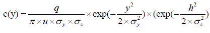
The Gaussian dispersion model assumed that the concentration of a pollutant in both the vertical and horizontal planes can be represented by a Gaussian distribution. According to the Gaussian model, the concentration in any point in 3D space is written in the following form 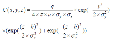(1).

(1)

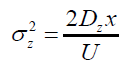
Where C is the pollutant concentration (g.m^-3), U represents the wind velocity (m.s^-1), q is the pollutant mass flow rate (g.s^-1), h denotes the chimney elevation (m) and σ_y and σ_z are the Gaussian standard deviations in the y and z direction. Based on the Pasquill Gifford stability class, the standard deviations σ_y and σ_z are calculated by the following (2) and (3) formula (Pasquill., 1961).

(2)

(3)

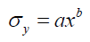
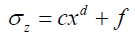
D_y and D_z are respectively the diffusion coefficients in the y and z direction and y is the distance from the source according to the y direction (km). These standard deviations are dependent on the length of the plume x-axis and on the meteorological condition. They are calculated based on the stability classification of the atmosphere (six categories (AF)), where A corresponds to extremely unstable and F Corresponds to very stable. (Eq. 4, 5).

(4)

(5)

The constants a, b, c, d and f are functions of the stability conditions of the atmosphere. These coefficients depending on stability class and distance from the emission source (Turner 1994).

To search the concentration at ground level (z=0) and knowing that the x-axis coincides with the axis panache, the equation (1) becomes (Cheng et al., 2015).

(6)

Results and Discussion

Spatial variation of concentration

With the chimney height H of 5 m, which is the real height of the existing chimney and knowing that the two factory chimneys are of the same height and the same rate of smoke, we calculated the concentration of pollutant from two chimneys and the total concentration by superposition. Then a comparison is made between the values of the determined concentration and Tunisian ambient air (Table 2). Fig. 2 shows that the concentration of CO peaks at 50 μgm^-3 approximate 50 m of the source and decreases to zero value at 400 m. It shows that the concentration of CO₂ is rapidly increased to reach its maximum of 185 mgm^-3 at 50 m then decreases to a value of 30 mgm^-3.

Table 2: National ambient air quality standards.

Fig. 2: Spatial evolution of [CO] and [CO₂].

Factors Influencing Pollutant Dispersion

Effect of the stack height

To highlight the effect of the stack height, we considered two sites with exactly the same conditions of temperature, pressure, flow, wind, and stack diameter, but different heights (5 m, 10 m, 30 m and 40 m), and the concentration variation as a function of x for the different heights are determined. We take the case where the velocity is equal to 4 m/s and the sun is strong and as a fuel an exhausted olive husk.

Note that the concentrations of pollutants at ground level for H=5 m are very high compared to the H/ height H=20 m (Fig. 3). The study of this phenomenon is of great interest in terms of pollution, because it is obvious that the dispersion from a stack of low height will be quite different from that obtained with a tall stack, which will benefit from more favorable dispersion. Thus, the use of tall stacks ensures good dispersion of gaseous pollutants, and leads to low concentrations of pollutants at ground level, but the solution to the pollution problem is not there, because the impact is just not only at the source, but it spreads to great distances using meteorological factors (wind etc..).

Fig. 3: Effect of stacks height on (a) CO and (b) CO₂ concentrations.

Effect of wind speed

To mark the effect of wind speed on the pollutant dispersion, exhausted olive husk is used as a fuel, and then we determine the concentration evolution of pollutant according to the wind speed. We fixed the distance from chimney to 50 m and the chimney height is 5 m (Fig. 4).

Fig. 4: Concentration versus wind speed for (a) CO and (b) CO₂ at different solar radiation.

There is a clear relationship between wind speed and the concentration levels of pollutants. Pollutant dispersion increases with wind speed and turbulence. A low wind therefore favors the accumulation of pollutants. When the wind speed is low, it can move away the pollutants with a certain zone, but, when the wind speed is high enough, it can carry a huge amount of pollutant from far away (wang and susuman., 2017). Indeed, when the wind speed increases, the dispersion, also, increases, and maximum concentrations go more away from the emission source. Dilution due to wind is even greater when the wind velocity is high. For a fixed rate of pollutants, the air rate, allowing dilution increases with velocity. In Fig 4(a) at wind speed equal to 2 m/s and at moderate solar radiation, the diffusion is poor and is accompanied by a lower atmospheric mixed layer, preventing the spread of pollutants and increasing the concentration (Zheng and yu, 2017).

Effect of fuel nature

We considered two sites with exactly the same conditions of temperature, pressure, flow, wind, and chimney diameter, but using as a fuel exhausted olive husk and natural gas. We took the case where the velocity is equal to 6 m/s and the sun is strong, and we determined the concentration variation as a function of x to highlight the effect of the fuel type on pollutant dispersion. The flow rates of the different components of the smoke out of the chimney using as a fuel gas are is given in Table 3.

Table 3: Mass flow of various pollutants out of stacks (for natural gas).

It is clear that the concentration of all pollutants produced by the combustion of exhausted olive husk is higher than that of these produced by the combustion of natural gas (Fig. 5). Using as a fuel exhausted olive husk, the [CO] increases until reaching its maximum at X=50 m, then it starts to decrease away from the source. Similarly, for natural gas, but the maximum of [CO] for this fuel is negligible compared to the use of exhausted olive husk. We can consider that natural gas is a clean gas generating little carbon dioxide and almost no other pollutants, since natural gas is mainly composed of methane (CH₄) and therefore much more hydrogen than carbon. For this reason, the rate of carbon dioxide (CO₂) from the water produced by the hydrogen in the form of vapor (H₂O) is less than that of other fuels. There is less carbon dioxide produced by caloric unit than other fuels.

Fig. 5: Effect of fuel nature on (a) CO and (b) CO₂ concentrations.

Effect of excess air

To determine the effect of the excess air in the dispersion of pollutants coming out of the chimney, the natural gas is used as a fuel, and varying the air flow entering the stove using a ventilator (Table 4). We took a wind velocity equal to 6 m/s, the sun is strong and X=50 m. It is seen from Fig. 6 that CO decreases when the excess air increases, unlike CO₂ increases with air excess. Indeed, promoting excess air, it provides more CO and OH radicals, so the next reaction is stimulated as:

CO + OH -> CO₂ + H°.

So CO disappears in favor of CO₂.

Moreover, increasing the excess air decreases the temperature and consequently inhibits reactions:

I) CO₂ + C-> 2CO: The reaction is promoted by raising the temperature and decreasing the pressure.

II) CO₂ + H2-> H₂O + CO: It is also favored by increasing the temperature (but remains independent of pressure). Thus, the amount of CO released increases with the richness of the mixture.

Fig. 6: Effect of excess air on CO and CO₂ concentrations.

Table 4: Analytical measurements on natural gas combustion fumes.

Effect of the combustion temperature

To determine the effect of the combustion temperature on pollutants dispersion leaving the chimney, natural gas is used as a fuel and varying the air flow entering the stove using a fan. CO increases gradually as the temperature increases, unlike CO₂ that decreases when T increases this is done in the following reaction (Fig. 7).

Fig. 7: Effect of the combustion temperature on CO and CO₂ concentrations.

Conclusion

In this work we evaluated first the pollutant concentration detected by the gas analyzer at ground level. The chimney height, the wind velocity, the solar radiation, the fuel nature, the air excess and the combustion temperature affect the pollutant dispersion. In fact, at wind speed equal to 2 m/s and at moderate solar radiation, the diffusion is poor and is accompanied by a lower atmospheric mixed layer, preventing the spread of pollutants and increasing the concentration. The use of tall stacks ensures good dispersion of gaseous pollutants and leads to low concentrations of pollutants at ground but the solution to the pollution problem is not there, because the impact is just not only at the source, but it spreads to great distances through meteorological factors.

References

1. Asadi, M., Asadollahfardi, G., Fakhraee, H. and Mirmohammadi, M. (2017). The comparison of Lagrangian and Gaussian models in predicting of air pollution emission using experimental study: A case study: Ammonia emission. Environ. Model. Assess. 22(1) : 27-36.
2. Brusca, S., Famoso, F., Lanzafame, R., Mauro, S., Garrano, A.M.C. and Monforte,P. (2016). Theoretical and experimental study of Gaussian plume model in small scale system. Energy Procedia. 101 : 58-65.
3. Cheng, G., Huang, G. G. and Dong, C. (2015). Synchronic interval Gaussian mixed- integer programming for air quality management. Sci Total Environ. 538 : 986-996.
4. Clark, P.U., Shakun, J.D., Marcott, S.A., Mix, A.C., Eby, M., Kulp, S., Levermann, A., Milne, G.A., Pfister, P.L., Santer, B.D. and Schrag, D.P. (2016). Consequences of twenty-first-century policy for multi- millennial climate and sea-level change. Nat Clim Chang. 6(4) : 360-369.
5. Connan, O., Smith, K., Organo, C., Solier, L., Maro, D. and Hébert, D. (2013).Comparison of RIMPUFF, HYSPLIT, ADMS atmospheric dispersion model outputs, using emergency response procedures, with 85Kr measurements made in the vicinity of nuclear reprocessing plant. J. Environ. Radioact. 124 : 266-277.
6. Conti, G.O., Heibati, B., Kloog, I., Fiore, M. and Ferrante, M. (2017). A review of AirQ Models and their applications for forecasting the air pollution healthoutcomes. Environ Sci Pollut Res Int. 24(7) : 6426-6445.
7. Dennis, R. L., Byun, D. W., Novak, J. H., Galluppi, K. J., Coats, C. J. and Vouk, M.A. (1996). The next generation of integrated air quality modeling: EPA's Models-3. Atmos Environ. 30(12) : 1925-1938.
8. Dey, S., Gupta, S., Sibanda, P., Chakraborty, A. and (2017). Spatio-temporal variation and futuristic emission scenario of ambient nitrogen dioxide over an urban area of eastern India using GIS and coupled AERMOD–WRF model. Plos One. 12(1) : e0170928.
9. Duo, B., Cui, L., Wang, Z., Li, R., Zhang, L., Fu, H. and Qiong, A. (2018).Observations of atmospheric pollutants at Lhasa during 2014–2015: Pollution status and the influence of meteorological factors. J Environ Sci . 63, 28-42.
10. Elperin, T., Fominykh, A. and Krasovitov, B. (2016). Effect of raindrop size distribution on scavenging of aerosol particles from Gaussian air pollution plumes and puffs in turbulent atmosphere. Process Saf Environ. 102 : 303-315.
11. Fallah-Shorshani, M., Shekarrizfard, M. and Hatzopoulou, M. (2017). Integrating a street-canyon model with a regional Gaussian dispersion model for improved characterisation of near-road air pollution. Atmos Environ. 153 : 21-31.
12. Grauer, S.J., Conrad, B.M., Miguel, R.B. and Daun, K.J. (2018). Gaussian model for emission rate measurement of heated plumes using hyperspectral data. J Quant Spectrosc Radiat Transf. 206 : 125-134.
13. Hong, Y.J., Huang, Y.C., Lee, I.L., Chiang, C.M., Lin, C. and Jeng, H.A. (2015).Assessment of volatile organic compounds and particulate matter in a dental clinic and health risks to clinic personnel. J. Environ. Sci. Health. 50(12) : 1205-1214.
14. http://www.meteo.tn/htmlen/accueil.php.
15. Huang, Y.D., Song, Y., Xu, X., He, W.R. and Kim, C. N. (2017). Impacts of upstream building height and stack location on pollutant dispersion from a rooftop stack. Aerosol Air Qual Res. 17(7) : 1837-1855.
16. Jaworski, M., Łapka, P. and Furmański, P. (2014). Numerical modelling and experimental studies of thermal behaviour of building integrated thermal energy storage unit in a form of a ceiling panel. Appl Energy .113 : 548-557.
17. Jo, J.H., Lim, J.H., Song, S.Y., Yeo, M.S. and Kim, K.W. (2007). Characteristics of pressure distribution and solution to the problems caused by stack effect in high- rise residential buildings. Build Environ. 42(1) : 263-277.
18. Lateb, M., Masson, C., Stathopoulos, T. and Bédard, C. (2011). Effect of stack height and exhaust velocity on pollutant dispersion in the wake of a building. Atmos Environ. 45(29) : 5150-5163.
19. Lee, J., Song, D. and Park, D. (2010). A study on the development and application of the E/V shaft cooling system to reduce stack effect in high-rise buildings. Building and Environment. 45(2) : 311-319.
20. Lelieveld, J., Evans, J.S., Fnais, M., Giannadaki, D. and Pozzer, A. (2015). The contribution of outdoor air pollution sources to premature mortality on a global scale. Nature. 525(7569) : 367-371.
21. Ma, X., Zhong, W., Feng, W. and Li, G. (2017). Modelling of pollutant dispersion with atmospheric instabilities in an industrial park. Powder Technol. 314 : 577- 588.
22. Milando, C. W., & Batterman, S. A. (2018). Operational evaluation of the RLINE dispersion model for studies of traffic-related air pollutants. Atmos Environ. 182 : 213-224.
23. Orru, H., Lövenheim, B., Johansson, C. and Forsberg, B. (2015). Potential health impacts of changes in air pollution exposure associated with moving traffic into a road tunnel. J Expo Anal Environ Epidemiol. 25(5) : 524-531.
24. Pasquill F. (1961) The estimation of the dispersion of windborne material. Meteor. Mag. 90 : 33-49.
25. Petelin, D., Grancharova, A. and Kocijan, J. (2013). Evolving Gaussian process models for prediction of ozone concentration in the air. Simul Model Pract Th. 33, 68-80.
26. Ristic, B., Gunatilaka, A. and Gailis, R. (2015). Achievable accuracy in Gaussian plume parameter estimation using a network of binary sensors. Information Fusion. 25, 42-48.
27. Rovira, J., Vilavert, L., Nadal, M., Schuhmacher, M. and Domingo, J.L. (2015).Temporal trends in the levels of metals, PCDD/Fs and PCBs in the vicinity of a municipal solid waste incinerator. Preliminary assessment of human health risks. Waste Manage. 43 : 168-175.
28. Shi, W.X., Ji, J., Sun, J.H., Lo, S.M., Li, L.J. and Yuan, X.Y. (2014). Experimental study on influence of stack effect on fire in the compartment adjacent to stairwell of high rise building. J. Civ. Eng. Manag. 20(1) : 121-131.
29. Talaiekhozani, A., Dokhani, M., Dehkordi, A.A., Eskandari, Z. and Rezania, S. (2018). Evaluation of emission inventory for the emitted pollutants from landfill of Borujerd and modeling of dispersion in the atmosphere. Urban Climate. 25 : 82-98.
30. Toja-Silva, F., Pregel-Hoderlein, C. and Chen, J. (2018). On the urban geometry generalization for CFD simulation of gas dispersion from chimneys: Comparison with Gaussian plume model. J Wind Eng Ind Aerod. 177 : 1-18.
31. Tomlin, A. S., Smalley, R.J., Tate, J.E., Barlow, J.F., Belcher, S.E., Arnold, S. J. and Robins, A. (2009). A field study of factors influencing the concentrations of a traffic-related pollutant in the vicinity of a complex urban junction. Atmos Environ. 43(32) : 5027-5037.
32. Tsuang, B.J. (2003). Quantification on the source/receptor relationship of primary pollutants and secondary aerosols by a Gaussian plume trajectory model: Part I- Theory. Atmos Environ. 37(28) : 3981-3991.
33. Turner, D.B. (1994). Workbook of atmospheric dispersion estimates: An introduction to dispersion modeling. CRC press.
34. Von Schneidemesser, E., Kuik, F., Mar, K.A. and Butler, T. (2017). Potential reductions in ambient NO2 concentrations from meeting diesel vehicle emissions standards. Environ. Res. Lett. 12(11) : 114025.
35. Wang, J. and Ogawa, S. (2015). Effects of meteorological conditions on PM2. 5 concentrations in Nagasaki, Japan. Int J Environ Res. 12(8) : 9089-9101.
36. Yu, J.Y., Cho, D.W. and Yu, K H. (2004). Evaluation of stack effect according to the shape and window area ratios of lobby in high-rise buildings: CTBUH. 10(13): 787-792.
37. Zeng, S. and Zhang, Y. (2017). The effect of meteorological elements on continuing heavy air pollution: A case study in the Chengdu area during the 2014 Spring Festival. Atmos Environ. 8(4) : 71.
38. Zeng, S. and Zhang, Y. (2014). Performance evaluation of AERMOD, CALPUFF, and legacy air dispersion models using the Winter Validation Tracer Study dataset. Atmos Environ. 89 : 707-720.