TEMPERATURE TREND ANALYSIS USING NONPARAMETRIC TEST: A CASE STUDY OF COIMBATORE CITY

Sathyanathan Rangarajan^*, Deeptha Thattia, Arun Subbiah, Abhishek Cherukuri, Tanmoy Akash Borah And Joel Kuncheria Joseph

Department of Civil Engineering, SRM University, Kattankulathur, TN 603203, India

*Corresponding Author:

Sathyanathan Rangarajan
E-mail: sathyanathan.r@ktr.srmuniv.ac.in

Received March 14, 2016; Accepted April 19, 2016

Visit for more related articles at Journal of Industrial Pollution Control

Abstract

Livelihoods of people, socio economic development and biodiversity as a whole are affected due to rise in temperature. In this study temperature trend analysis is studied for the Coimbatore district, which witnessed a speedy industrial and business growthfrom the 1920s. Well established nonparametric tests like Mann-Kendall, Sen’s slope and Pettitt’s test are applied to the maximum and minimum temperatures to find the nature of trend and detect the change point. The result of the analysis confirmed an increasing trend in both minimum and maximum temperatures in all the months and seasons post 1950.

Keywords

Ultra High Performance Concrete (UHPC), Hybrid steel fiber, Compressive strength, Flexural strength, Load – Deflection Relationship, Stress-strain relationship modulus of elasticity, Modulus of toughness, Ductility of UHPC

Introduction

Population growth, industrialization, and global warming are the root cause for rise in temperatures (IPCC, 2013; Rao, et al., 2016) There has been a drastic change in global climatic conditions in recent years. Global land evapotranspiration influence the variation in land precipitation (Qian, et al., 2006) which results in frequent extreme weather events and risks (Briffa, et al., 2009; Vasiliades, et al., 2009). Many have studied and analyzed the trends in long term temperature, its interannual, seasonal and decadal variability by using different nonparametric tests (Bhutiyani, et al., 2008; Jaiswal, et al., 2015; Jagannathan and Parthasarathy, 1973; Xavier, 2006; Wijngaard, et al., 2003). Though various statistical methods are employed by researchers for analyzing trends and change point detection, nonparametric methods are preferred over parametric ones. Since parametric tests are mostly appropriate for normally distributed data, if the assumed data distribution deviates considerably from the standard, then the nonparametric test gives much better results that the parametric one (Hirsch, et al., 1992; Pettitt, 1979). In this study, the trend and change point detection is examined for theminimum and maximum temperature series of Coimbatore district by employing different nonparametric tests. Man- Kendall’s test and Sen’s slope test are used for trend analysis and Pettitt’s test is employedfor change point detection.

 Study Area

Coimbatore district is situated in the northwestern part of Tamil Nadu. It lies between 10°13'4" North and 11° 24'5" North latitudes and 76°39'25" East and 77°18'26" East longitudes. It is one among the industrially developed and commercially vibrant districts of Tamil Nadu. The district is situated on the banks of river Noyyal, a tributary of the river Cauveryand is bounded by Tiruppur district in the east, Nilgiris district in the north, Erode district in the northeast, Palghat district and Idukki district of the neighboring state of Kerala in the west and south, respectively. The gradient of the district decreases gradually from west to east. The district was bifurcated into Coimbatore and Erode districts in the year 1979 and presently it consists of two revenue divisions and six taluks. It has a high concentration of small, medium and large scale industries. It is also called as the Manchester of South India because of its well-developed textile, commerce and other industrial areas. The district gained an economic boom between the years 1920 and 1930 due to decline of cotton industry in Mumbai (Dhanalakshmi and Priyatharsini; 2015; www.coimbatore.nic.in) (Figure 1).

Figure 1: Location map of Coimbatore district, Tamil Nadu, India.

Box plot showing the characteristics of minimum and maximum temperatures is presented in (Figure 2 and Figure 3).

Figure 2: Box plot of monthly minimum temperatures averaged over years.

Figure 3: Box plot of monthly maximum temperatures averaged over years.

Methodology

Mann-Kendall’s Test

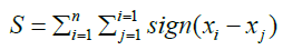
The nonparametric Mann-Kendall test is commonly employed to detect monotonic trends in series of environmental data, climate data or hydrological data. The null hypothesis, H₀, is that the data come from a population with independent realizations and are identically distributed. The alternative hypothesis, H_A, is that the data follow a monotonic trend (Karmeshu, 2012; Libiseller and Grimvall, 2002; Menne and Williams, 2005). The Mann- Kendall test statistic is calculated according to:

(1)

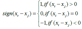
where n is the total length of data, x_i and x_j are two generic sequential data values, and function sign (x_i—x_j ) assumes the following values

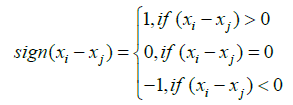(2)

Pettitt’s Test

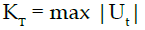
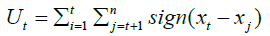
The approach after Pettitt is commonly applied to detect a single change-point in hydrological series or climate series with continuous data. It tests the H₀: The T variables follow one or more distributions that have the same location parameter (no change), against the alternative: a change point exists (Dhanalakshmi and Priyatharsini, 2015; Menne and Williams, 2005). The non-parametric statistic is defined as:

(3)

Where

(4)

(5)

The test statistic counts the number of times a member of the first sample exceeds the member of second sample. The null hypothesis of the Pettitt’s test is the absence of a change point.

Sen’s Slope Test

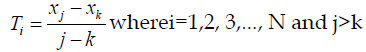
This test computes both the slope (i.e., linear rate of change) and intercept according to Sen’s method. First, a set of linear slopes is calculated as follows:

(6)

where x₁, x₂, x₃, …, x_j, x_k, …, x_n are the data values and the median of N values of Ti series can be obtained as Sen’s estimator of slope (Libiseller and Grimvall, 2002).

Analysis of Results

Detection of trend

The monthly temperature data from 1902–2002 is obtained from the Indian Meteorological Department (IMD) site India Water Portal (http://www.indiawaterportal.org/metdata) (Mitchell, et al., 2004) and the seasonal classification for the analysis was followed as per Indian Meteorological Department (IMD) viz. winter (January–February), summer (March–May), southwest monsoon (June–September) and northeast monsoon (October–December). For the determination of trend, Mann-Kendall’s test has been applied on the data series of maximum and minimum temperatures. The trend is detected based on the z value at the given significance level. If the z value is greater than the significance level, the null hypothesis (H0) is rejected and the rejection of H0 indicates that there is a trend in the time series. The results of Mann-Kendall test statistic is presented in Table 1. The test results showed significant increasing trend in both maximum and minimum temperatures in all the months and seasons barring August.

Table 1: Results of Mann Kendall test statistics (Z) during 1902–2002

To determine the change point for the maximum and minimum temperature series, Pettitt’s test has been applied. The results are presented in Table 2. It is observed that the change point of minimum and maximum temperature series of all the months and seasons varies between the years 1950 and 1980. A number of trial runs were performed to find the exact change point by dividing the entire span with respect to the results obtained in Table 2. Based on the test outcomes, the entire span of 1902–2002 (P-1) is divided into two periods viz. P-2 (1902–1951) andP- 3 (1941–2002) for which trend analysis is performed again to substantiate the change point.

Table 2: Results of change point analysis

Mann-Kendall’s test results for P-2 and P-3 are presented in Table 3 and Table 4. For the minimum temperature series (Table 3), P-2 (1902–1951) period shows significant trend for January and April and no significant trend is identified for the other months and seasons. For the period P-3 (1941–2002), an upward trend is witnessed for all the months and seasons. An increasing trend is also witnessed for the maximum temperature series for the period P-3 (Table 4). Thus the trend analysis confirmed a significant rising trend in all monthly and seasonal series during the period 1941–2002 (P-3). The significant increase in temperature might be due to the growth of industrialization in Coimbatore district post 1930s. The annual series of minimum and maximum temperatures when plotted and fitted linearly showed that both series exhibited strong rising trend during the period P-3, while an insignificant trend was detected in P-2 (Figure 4).

Figure 4: Fitting of linear trends in minimum and maximum temperature series.

Table 3: Mann-Kendall’s test and trends in different periods of minimum temperature

Table 4: Mann-Kendall’s test and trend in different periods of maximum temperature

Sens’s Slope Estimator Test

Sen’s slope was computed to know the prevailing trends in monthly and seasonal series of minimum and maximum temperatures. The Sen’s slope parameters for minimum and maximum temperature series are presented in Table 5. The analysis of Sen’s slope estimator clearly indicated a positive trend in P-3 (1941–2002) period for both maximum and minimum temperature series while the same was either negative or with a minimalpositive value in P-2 (1902–1950).

Table 5: Sen’s Slope for minimum and maximum temperature

Conclusion

Rapid industrialization, global warming and other meteorological factors play a significant role in the rise in temperature. This has an apparent effect globally which might be in the form of increased precipitation rising sea level, retreating glaciers etc. In the present study, trend analysis was studied by applying Mann-Kendall’s test and the change point was found by using Pettitt’s test for the maximum and minimum temperature series of Coimbatore district. The result of trend analysis by Mann-Kendall and Sen’s slope showed a positive trend in the minimum and maximum temperature series between 1902 and 2002. The period P-2 (1902–1950) witnessed an insignificant trend while period P-3 (1941–2002) showed significant rising trend in temperature. The increase in temperature after 1940 is also substantiated by the Sen’s slope values. The increase in temperature might change the hydrological cycle which will eventually affect the crop production and agricultural activities. Analyses such as these will help in proper decision-making in water resources.

References

1. Bhutiyani, M.R., Kale, V.S. and Pawar, N.J. (2008). Changing stream flow patterns in the rivers of Northwestern Himalaya: Implications of global warming in the 20th century. Current Science. 95 : 618-626.
2. Briffa, K.R., Schrier, v.G. and Jones, P.D. (2009). Wet and dry summers in Europe since 1750: Evidence of increasing drought. Int. J. Climatol. 29 : 1894-1905.
3. Dhanalakshmi, B. and Priyatharsini, P. (2015). An assessment of fresh water piscine diversity in selected wetlands in Coimbatore District, Tamilnadu, India��?A Preliminary Study. Open Access Library Journal. 2 : 1-6.
4. Hirsch, R.M., Helsel, D.R., Cohn, T.A., Gilroy, E.J. and Maidment, D.R. (1992). Statistical analysis of hydrologic data. Handbook of Hydrology. 17��?21.
5. IPCC. (2013) Climate Change 2013: The physical science basis. Contribution of Working Group I to the Fifth Assessment Report of the Intergovernmental Panel on Climate Change. Cambridge University Press, Cambridge and New York.
6. Jagannathan, P. and Parthasarathy, B. (1973). Trends and periodicities of rainfall over India. Monthly Weather Review. 101 : 691��?700.
7. Jaiswa, R.K., Lohani, A.K. and Tiwari, H.L. (2015). Study of change point and trend in temperature of Raipur in Chhattisgarh (India). Indian Water Resources society. 35 : 39-47.
8. Karmeshu, N. (2012). Trend detection in annual temperature and precipitation using the Mann Kendall Test��?A case study to assess climate change on select states in the Northeastern United States. Master of Environment Studies Capstone project, University of Pennsylvania USA.
9. Libiseller, C. and Grimvall, A. (2002). Performance of partial Mann-Kendall tests for trend detection in the presence of covariates. Environmetrics. 13 : 71-84.
10. Menne, J.M. and Williams, C.N.J. (2005). Detection of undocumented change points using multiple test statistics and composite reference series. J Clim. 18 : 4271-4286.
11. Mitchell, T.D., Carter, T.R., Jones, P.D, Hulme, M. and New, M. (2004). A comprehensive set of high-resolution grids of monthly climate for Europe and the globe: the observed record (1901��?2000) and 16 scenarios (2001��?2100). Tyndall Working Paper 55, Tyndall Centre, UEA, Norwich, UK.
12. Pettitt, A.N. (1979). A non-parametric approach to the change-point detection. Appl.Stat. 28 : 126-135.
13. Qian T, Dai, A., Kevin, E.T. and Keith W.O. (2006). Simulation of global land surface conditions from 1948��?2004: Part I. Forcing data and evaluations. J Hydrometeorol. 7 : 953-975
14. Rao, V.B., Franchito, S.H., Ger�?³lamo. R.O.P., Giarolla, E., Ramakrishna, S.S.V.S., Rao, B.R.S. and Naidu, C.V. (2016). Himalayan warming and climate change in India. American Journal of Climate Change. 5 : 558-574.
15. Vasiliades, L., Loukas, A. and Patsonas, G. (2009). Evaluation of a statistical downscaling procedure for the estimation of climate change impacts on droughts. Nat. Hazards Earth Syst. Sci. 9 : 879-894.
16. Wijngaard, J.B., Kleink, T.A.M.G. and Konnen, G.P. (2003). Homogeneity of 20th Century European Daily Temperature and Precipitation Series. Int. J Climatol. 23 : 679-692.
17. www.coimbatore.nic.in .
18. Xavier, P.K. (2006). Increasing trend of extreme rain events over India in a warming environment. Science. 314 : 1442-1445.